Data Representation in Computer: Number Systems, Characters, Audio, Image and Video
What is data representation in computer, number systems, binary number system, octal number system, decimal number system, hexadecimal number system, data representation of characters.
It stands for Extended Binary Coded Decimal Interchange Code. This is similar to ASCII and is an 8-bit code used in computers manufactured by International Business Machines (IBM). It is capable of encoding 256 characters.
Using 8-bit ASCII we can represent only 256 characters. This cannot represent all characters of written languages of the world and other symbols. Unicode is developed to resolve this problem. It aims to provide a standard character encoding scheme, which is universal and efficient.

Browse Books

February 2018
- Bentham Science Publishers
Save to Binder
Introduction to Computer Data Representation introduces readers to the representation of data within computers. Starting from basic principles of number representation in computers, the book covers the representation of both integer and floating point numbers, and characters or text. It comprehensively explains the main techniques of computer arithmetic and logical manipulation. The book also features chapters covering the less usual topics of basic checksums and universal or variable length representations for integers, with additional coverage of Gray Codes, BCD codes and logarithmic representations. The description of character coding includes information on both MIME and Unicode formats. Introduction to Computer Data Representation also includes historical aspects of data representation, explaining some of the steps that developers took (and the mistakes they made) that led to the present, well-defined and accepted standards of data representation techniques. The book serves as a primer for advanced computer science graduates and a handy reference for anyone wanting to learn about numbers and data representation in computers.
- Publication Years 1984 - 2018
- Publication counts 20
- Citation count 68
- Available for Download 1
- Downloads (cumulative) 125
- Downloads (12 months) 14
- Downloads (6 weeks) 3
- Average Downloads per Article 125
- Average Citation per Article 3
Recommendations
Mathematical representation of computer character data, introduction to computer graphics: using java 2d and 3d (undergraduate topics in computer science), computer representation of real numbers.
Hwang's[1] model for the computer representation of real numbers is extended to explicitly distinguish between the representational system used to denote real numbers and the internal encoding of the digits of the representation in the computer memory. ...
Export Citations
- Please download or close your previous search result export first before starting a new bulk export. Preview is not available. By clicking download, a status dialog will open to start the export process. The process may take a few minutes but once it finishes a file will be downloadable from your browser. You may continue to browse the DL while the export process is in progress. Download
- Download citation
- Copy citation
We are preparing your search results for download ...
We will inform you here when the file is ready.
Your file of search results citations is now ready.
Your search export query has expired. Please try again.
- Books by Title
- Books by Subject
- Book Series by Title
Book Categories
- Open Access Books
- Video Books
- Forthcoming Titles
- Forthcoming Series
- Book Catalog
Future Attractions
- Future Books
- Future Series
For Reviewers
- Pre-publication Peer Review
- Post-publication Book Review
For Buyers and Librarians
- Purchase and Ordering Procedure
- End User License Agreement
- Register for New Book Alert
For Authors and Editors
- Submission Guidelines
- Animated Abstracts
- Manuscript Organization
- Guideline for Conference Proceedings
- Publishing Process
- Editorial Policies
- Copyright and Permissions
- Peer Review Workflow
- Offers and Services
- Tips to Promote Books
- Book Proposal Submission Form
Marketing Opportunities
- Conference Discounts on Books
- Exhibit Schedule
- Media Partners
- Partnering Events
Advertising
- Advertise With Us
- Journals and Books Catalog
General Queries
- Introduction of Bentham Books
- Author Incentives
- Purchase and Order
- Read and Search
- Publishing Contract
- Copyright and Permission for Reproduction
- Discounts and Offers
- Submit Proposals and Manuscripts
Site Breadcrumb

Introduction to Computer Data Representation
Introduction.
Introduction to Computer Data Representation introduces readers to the representation of data within computers. Starting from basic principles of number representation in computers, the book covers the representation of both integer and floating point numbers, and characters or text. It comprehensively explains the main techniques of computer arithmetic and logical manipulation. The book also features chapters covering the less usual topics of basic checksums and ‘universal’ or variable length representations for integers, with additional coverage of Gray Codes, BCD codes and logarithmic representations. The description of character coding includes information on both MIME and Unicode formats. Introduction to Computer Data Representation also includes historical aspects of data representation, explaining some of the steps that developers took (and the mistakes they made) that led to the present, well-defined and accepted standards of data representation techniques. The book serves as a primer for advanced computer science graduates and a handy reference for anyone wanting to learn about numbers and data representation in computers.
- Contributors
It is my great pleasure to recommend this excellent book written by my friend and colleague, Professor Peter Fenwick. During the eleven years I have known him, we have had many a discussion, often touching on topics covered here. Though this is the closest we have come to a collaboration I have little doubt that had we met earlier in our careers we would have collaborated extensively.
A major contribution of this book is to bring a historical perspective to many topics that are so widely accepted that it might not be obvious there were choices to be made. The binary representation of numbers was so obvious even in the 1940s that Burks, Goldstine and von Neumann are said to have “adopted it seemingly without discussion”. But Burks et al considered floating point representation, then argued against supporting it. Long ago I heard it claimed that von Neumann believed any mathematician ”worth his salt” should be able to specify floating point computations using only integers. In any case, floating point only came into its own in the 1980s, with the broad acceptance of the IEEE standards. Professor Fenwick shows great insight into why it took decades to get right something as basic as the representation of numbers.
A second important contribution is discussion of the introduction of redundancy to increase reliability in the presence of errors: check sums and variable-length (universal) codes. While simple check sums are frequently discussed, I know of no comparable source for a general discussion of Universal codes, an important but somewhat obscure subject.
I agree with Professor Fenwick's quote, that “everybody thinks they know” about these topics, but there are big holes, even today. Surely most of us have superficial knowledge that fails us when we really need to work through the details. This book covers a huge range of material, thoroughly and concisely. I have taught a good bit of the material, but I learned much, even in areas where I claim some expertise. The book displays a deep understanding of the many and varied requirements for digital representation of information, from the obvious integers and floating point, to Zeckendorf representations and Gray codes; from 2's complement to logarithmic arithmetic; from Elias and Levenstein codes to Rice and Golomb codes and on to Ternary Comma and Fibonacci codes.
In addition to the plethora of ways to represent numbers, it also covers representation of characters and strings. While the book will serve very well as a reference, it is also fascinating reading. Many pages are devoted to obscure topics, interesting largely because of their place in history, but outside the domain of a classic textbook on computer organization or architecture. These are perhaps the most important sections, precisely because they had to be understood and discarded to get us where we are now.
This book definitely does not qualify for the subtitle, “Data Representation for Dummies”. While it quickly surveys common forms of representation, the pace and breadth will bewilder the true novice. On occasions, it uses terms unfamiliar (at least to an American), requiring another source. Appropriately, Professor Fenwick acknowledges the role of Wikipedia, which covers rather more topics than his book, but certainly not as coherently.
The author has a wry, if somewhat subtle, sense of humour which often surfaces unexpectedly: it's a bit of a stretch, but of course the description and figure regarding Gray codes include a “grey area”!
Discussion of the roles and interaction of precision, accuracy and range is superb. Floating point representation is highly precise, so why is it dangerous for use in financial calculations? Professor Fenwick points out something that had not occurred to me: a “quite ordinary calculator” is capable of more precise arithmetic than a 32-bit [IEEE single-precision] floating point computation. That explains why the calculator “app” on my iPad has both less range, and less precision, than the HP calculator I bought 35 years ago!
A topic rarely covered so clearly is “unwarranted precision”, the process of using a precise mathematical operation to apparently increase accuracy (significant digits) of a number. Professor Fenwick points out confusion over precision created by the fact that the speed of light is so close to 300,000,000 metres per second—and the fact that scientific notation provides information about the accuracy of a value (pp. 106-107). I especially liked his discussion of the sins of the popular press, for example, by apparently increasing precision in the process of converting units: an altitude “10,000 feet”—accurate to, say, ±100 metres—becomes the apparently more precise, but inaccurate, “3 048 metres”. It is unfortunate that the general level of this book is beyond comprehension for most journalists!
In short, this is a fascinating book that will appeal to many because of its authoritative exploration of how we represent information. But it will also serve as a reference for those requiring—or simply enjoying—the ability to choose efficient representations that lead to accurate results. It's a good read, and a great book to keep handy.
James R. Goodman , United States of America Fellow IEEE, Fellow ACM, 2013 Eckert-Mauchly Award
RELATED BOOKS


- Data representation
Bytes of memory
- Abstract machine
Unsigned integer representation
Signed integer representation, pointer representation, array representation, compiler layout, array access performance, collection representation.
- Consequences of size and alignment rules
Uninitialized objects
Pointer arithmetic, undefined behavior.
- Computer arithmetic
Arena allocation
This course is about learning how computers work, from the perspective of systems software: what makes programs work fast or slow, and how properties of the machines we program impact the programs we write. We want to communicate ideas, tools, and an experimental approach.
The course divides into six units:
- Assembly & machine programming
- Storage & caching
- Kernel programming
- Process management
- Concurrency
The first unit, data representation , is all about how different forms of data can be represented in terms the computer can understand.
Computer memory is kind of like a Lite Brite.

A Lite Brite is big black backlit pegboard coupled with a supply of colored pegs, in a limited set of colors. You can plug in the pegs to make all kinds of designs. A computer’s memory is like a vast pegboard where each slot holds one of 256 different colors. The colors are numbered 0 through 255, so each slot holds one byte . (A byte is a number between 0 and 255, inclusive.)
A slot of computer memory is identified by its address . On a computer with M bytes of memory, and therefore M slots, you can think of the address as a number between 0 and M −1. My laptop has 16 gibibytes of memory, so M = 16×2 30 = 2 34 = 17,179,869,184 = 0x4'0000'0000 —a very large number!
The problem of data representation is the problem of representing all the concepts we might want to use in programming—integers, fractions, real numbers, sets, pictures, texts, buildings, animal species, relationships—using the limited medium of addresses and bytes.
Powers of ten and powers of two. Digital computers love the number two and all powers of two. The electronics of digital computers are based on the bit , the smallest unit of storage, which a base-two digit: either 0 or 1. More complicated objects are represented by collections of bits. This choice has many scale and error-correction advantages. It also refracts upwards to larger choices, and even into terminology. Memory chips, for example, have capacities based on large powers of two, such as 2 30 bytes. Since 2 10 = 1024 is pretty close to 1,000, 2 20 = 1,048,576 is pretty close to a million, and 2 30 = 1,073,741,824 is pretty close to a billion, it’s common to refer to 2 30 bytes of memory as “a giga byte,” even though that actually means 10 9 = 1,000,000,000 bytes. But for greater precision, there are terms that explicitly signal the use of powers of two. 2 30 is a gibibyte : the “-bi-” component means “binary.”
Virtual memory. Modern computers actually abstract their memory spaces using a technique called virtual memory . The lowest-level kind of address, called a physical address , really does take on values between 0 and M −1. However, even on a 16GiB machine like my laptop, the addresses we see in programs can take on values like 0x7ffe'ea2c'aa67 that are much larger than M −1 = 0x3'ffff'ffff . The addresses used in programs are called virtual addresses . They’re incredibly useful for protection: since different running programs have logically independent address spaces, it’s much less likely that a bug in one program will crash the whole machine. We’ll learn about virtual memory in much more depth in the kernel unit ; the distinction between virtual and physical addresses is not as critical for data representation.
Most programming languages prevent their users from directly accessing memory. But not C and C++! These languages let you access any byte of memory with a valid address. This is powerful; it is also very dangerous. But it lets us get a hands-on view of how computers really work.
C++ programs accomplish their work by constructing, examining, and modifying objects . An object is a region of data storage that contains a value, such as the integer 12. (The standard specifically says “a region of data storage in the execution environment, the contents of which can represent values”.) Memory is called “memory” because it remembers object values.
In this unit, we often use functions called hexdump to examine memory. These functions are defined in hexdump.cc . hexdump_object(x) prints out the bytes of memory that comprise an object named x , while hexdump(ptr, size) prints out the size bytes of memory starting at a pointer ptr .
For example, in datarep1/add.cc , we might use hexdump_object to examine the memory used to represent some integers:
This display reports that a , b , and c are each four bytes long; that a , b , and c are located at different, nonoverlapping addresses (the long hex number in the first column); and shows us how the numbers 1, 2, and 3 are represented in terms of bytes. (More on that later.)
The compiler, hardware, and standard together define how objects of different types map to bytes. Each object uses a contiguous range of addresses (and thus bytes), and objects never overlap (objects that are active simultaneously are always stored in distinct address ranges).
Since C and C++ are designed to help software interface with hardware devices, their standards are transparent about how objects are stored. A C++ program can ask how big an object is using the sizeof keyword. sizeof(T) returns the number of bytes in the representation of an object of type T , and sizeof(x) returns the size of object x . The result of sizeof is a value of type size_t , which is an unsigned integer type large enough to hold any representable size. On 64-bit architectures, such as x86-64 (our focus in this course), size_t can hold numbers between 0 and 2 64 –1.
Qualitatively different objects may have the same data representation. For example, the following three objects have the same data representation on x86-64, which you can verify using hexdump :
In C and C++, you can’t reliably tell the type of an object by looking at the contents of its memory. That’s why tricks like our different addf*.cc functions work.
An object can have many names. For example, here, local and *ptr refer to the same object:
The different names for an object are sometimes called aliases .
There are five objects here:
- ch1 , a global variable
- ch2 , a constant (non-modifiable) global variable
- ch3 , a local variable
- ch4 , a local variable
- the anonymous storage allocated by new char and accessed by *ch4
Each object has a lifetime , which is called storage duration by the standard. There are three different kinds of lifetime.
- static lifetime: The object lasts as long as the program runs. ( ch1 , ch2 )
- automatic lifetime: The compiler allocates and destroys the object automatically as the program runs, based on the object’s scope (the region of the program in which it is meaningful). ( ch3 , ch4 )
- dynamic lifetime: The programmer allocates and destroys the object explicitly. ( *allocated_ch )
Objects with dynamic lifetime aren’t easy to use correctly. Dynamic lifetime causes many serious problems in C programs, including memory leaks, use-after-free, double-free, and so forth. Those serious problems cause undefined behavior and play a “disastrously central role” in “our ongoing computer security nightmare” . But dynamic lifetime is critically important. Only with dynamic lifetime can you construct an object whose size isn’t known at compile time, or construct an object that outlives the function that created it.
The compiler and operating system work together to put objects at different addresses. A program’s address space (which is the range of addresses accessible to a program) divides into regions called segments . Objects with different lifetimes are placed into different segments. The most important segments are:
- Code (also known as text or read-only data ). Contains instructions and constant global objects. Unmodifiable; static lifetime.
- Data . Contains non-constant global objects. Modifiable; static lifetime.
- Heap . Modifiable; dynamic lifetime.
- Stack . Modifiable; automatic lifetime.
The compiler decides on a segment for each object based on its lifetime. The final compiler phase, which is called the linker , then groups all the program’s objects by segment (so, for instance, global variables from different compiler runs are grouped together into a single segment). Finally, when a program runs, the operating system loads the segments into memory. (The stack and heap segments grow on demand.)
We can use a program to investigate where objects with different lifetimes are stored. (See cs61-lectures/datarep2/mexplore0.cc .) This shows address ranges like this:
Object declaration | Lifetime | Segment | Example address range |
|---|---|---|---|
Constant global | Static | Code (or Text) | 0x40'0000 (≈1 × 2 ) |
Global | Static | Data | 0x60'0000 (≈1.5 × 2 ) |
Local | Automatic | Stack | 0x7fff'448d'0000 (≈2 = 2 × 2 ) |
Anonymous, returned by | Dynamic | Heap | 0x1a0'0000 (≈8 × 2 ) |
Constant global data and global data have the same lifetime, but are stored in different segments. The operating system uses different segments so it can prevent the program from modifying constants. It marks the code segment, which contains functions (instructions) and constant global data, as read-only, and any attempt to modify code-segment memory causes a crash (a “Segmentation violation”).
An executable is normally at least as big as the static-lifetime data (the code and data segments together). Since all that data must be in memory for the entire lifetime of the program, it’s written to disk and then loaded by the OS before the program starts running. There is an exception, however: the “bss” segment is used to hold modifiable static-lifetime data with initial value zero. Such data is common, since all static-lifetime data is initialized to zero unless otherwise specified in the program text. Rather than storing a bunch of zeros in the object files and executable, the compiler and linker simply track the location and size of all zero-initialized global data. The operating system sets this memory to zero during the program load process. Clearing memory is faster than loading data from disk, so this optimization saves both time (the program loads faster) and space (the executable is smaller).
Abstract machine and hardware
Programming involves turning an idea into hardware instructions. This transformation happens in multiple steps, some you control and some controlled by other programs.
First you have an idea , like “I want to make a flappy bird iPhone game.” The computer can’t (yet) understand that idea. So you transform the idea into a program , written in some programming language . This process is called programming.
A C++ program actually runs on an abstract machine . The behavior of this machine is defined by the C++ standard , a technical document. This document is supposed to be so precisely written as to have an exact mathematical meaning, defining exactly how every C++ program behaves. But the document can’t run programs!
C++ programs run on hardware (mostly), and the hardware determines what behavior we see. Mapping abstract machine behavior to instructions on real hardware is the task of the C++ compiler (and the standard library and operating system). A C++ compiler is correct if and only if it translates each correct program to instructions that simulate the expected behavior of the abstract machine.
This same rough series of transformations happens for any programming language, although some languages use interpreters rather than compilers.
A bit is the fundamental unit of digital information: it’s either 0 or 1.
C++ manages memory in units of bytes —8 contiguous bits that together can represent numbers between 0 and 255. C’s unit for a byte is char : the abstract machine says a byte is stored in char . That means an unsigned char holds values in the inclusive range [0, 255].
The C++ standard actually doesn’t require that a byte hold 8 bits, and on some crazy machines from decades ago , bytes could hold nine bits! (!?)
But larger numbers, such as 258, don’t fit in a single byte. To represent such numbers, we must use multiple bytes. The abstract machine doesn’t specify exactly how this is done—it’s the compiler and hardware’s job to implement a choice. But modern computers always use place–value notation , just like in decimal numbers. In decimal, the number 258 is written with three digits, the meanings of which are determined both by the digit and by their place in the overall number:
\[ 258 = 2\times10^2 + 5\times10^1 + 8\times10^0 \]
The computer uses base 256 instead of base 10. Two adjacent bytes can represent numbers between 0 and \(255\times256+255 = 65535 = 2^{16}-1\) , inclusive. A number larger than this would take three or more bytes.
\[ 258 = 1\times256^1 + 2\times256^0 \]
On x86-64, the ones place, the least significant byte, is on the left, at the lowest address in the contiguous two-byte range used to represent the integer. This is the opposite of how decimal numbers are written: decimal numbers put the most significant digit on the left. The representation choice of putting the least-significant byte in the lowest address is called little-endian representation. x86-64 uses little-endian representation.
Some computers actually store multi-byte integers the other way, with the most significant byte stored in the lowest address; that’s called big-endian representation. The Internet’s fundamental protocols, such as IP and TCP, also use big-endian order for multi-byte integers, so big-endian is also called “network” byte order.
The C++ standard defines five fundamental unsigned integer types, along with relationships among their sizes. Here they are, along with their actual sizes and ranges on x86-64:
Type | Size | Size | Range |
|---|---|---|---|
| 1 | 1 | [0, 255] = [0, 2 −1] |
| ≥1 | 2 | [0, 65,535] = [0, 2 −1] |
| ≥ | 4 | [0, 4,294,967,295] = [0, 2 −1] |
| ≥ | 8 | [0, 18,446,744,073,709,551,615] = [0, 2 −1] |
| ≥ | 8 | [0, 18,446,744,073,709,551,615] = [0, 2 −1] |
Other architectures and operating systems implement different ranges for these types. For instance, on IA32 machines like Intel’s Pentium (the 32-bit processors that predated x86-64), sizeof(long) was 4, not 8.
Note that all values of a smaller unsigned integer type can fit in any larger unsigned integer type. When a value of a larger unsigned integer type is placed in a smaller unsigned integer object, however, not every value fits; for instance, the unsigned short value 258 doesn’t fit in an unsigned char x . When this occurs, the C++ abstract machine requires that the smaller object’s value equals the least -significant bits of the larger value (so x will equal 2).
In addition to these types, whose sizes can vary, C++ has integer types whose sizes are fixed. uint8_t , uint16_t , uint32_t , and uint64_t define 8-bit, 16-bit, 32-bit, and 64-bit unsigned integers, respectively; on x86-64, these correspond to unsigned char , unsigned short , unsigned int , and unsigned long .
This general procedure is used to represent a multi-byte integer in memory.
- Write the large integer in hexadecimal format, including all leading zeros required by the type size. For example, the unsigned value 65534 would be written 0x0000FFFE . There will be twice as many hexadecimal digits as sizeof(TYPE) .
- Divide the integer into its component bytes, which are its digits in base 256. In our example, they are, from most to least significant, 0x00, 0x00, 0xFF, and 0xFE.
In little-endian representation, the bytes are stored in memory from least to most significant. If our example was stored at address 0x30, we would have:
In big-endian representation, the bytes are stored in the reverse order.
Computers are often fastest at dealing with fixed-length numbers, rather than variable-length numbers, and processor internals are organized around a fixed word size . A word is the natural unit of data used by a processor design . In most modern processors, this natural unit is 8 bytes or 64 bits , because this is the power-of-two number of bytes big enough to hold those processors’ memory addresses. Many older processors could access less memory and had correspondingly smaller word sizes, such as 4 bytes (32 bits).
The best representation for signed integers—and the choice made by x86-64, and by the C++20 abstract machine—is two’s complement . Two’s complement representation is based on this principle: Addition and subtraction of signed integers shall use the same instructions as addition and subtraction of unsigned integers.
To see what this means, let’s think about what -x should mean when x is an unsigned integer. Wait, negative unsigned?! This isn’t an oxymoron because C++ uses modular arithmetic for unsigned integers: the result of an arithmetic operation on unsigned values is always taken modulo 2 B , where B is the number of bits in the unsigned value type. Thus, on x86-64,
-x is simply the number that, when added to x , yields 0 (mod 2 B ). For example, when unsigned x = 0xFFFFFFFFU , then -x == 1U , since x + -x equals zero (mod 2 32 ).
To obtain -x , we flip all the bits in x (an operation written ~x ) and then add 1. To see why, consider the bit representations. What is x + (~x + 1) ? Well, (~x) i (the i th bit of ~x ) is 1 whenever x i is 0, and vice versa. That means that every bit of x + ~x is 1 (there are no carries), and x + ~x is the largest unsigned integer, with value 2 B -1. If we add 1 to this, we get 2 B . Which is 0 (mod 2 B )! The highest “carry” bit is dropped, leaving zero.
Two’s complement arithmetic uses half of the unsigned integer representations for negative numbers. A two’s-complement signed integer with B bits has the following values:
- If the most-significant bit is 1, the represented number is negative. Specifically, the represented number is – (~x + 1) , where the outer negative sign is mathematical negation (not computer arithmetic).
- If every bit is 0, the represented number is 0.
- If the most-significant but is 0 but some other bit is 1, the represented number is positive.
The most significant bit is also called the sign bit , because if it is 1, then the represented value depends on the signedness of the type (and that value is negative for signed types).
Another way to think about two’s-complement is that, for B -bit integers, the most-significant bit has place value 2 B –1 in unsigned arithmetic and negative 2 B –1 in signed arithmetic. All other bits have the same place values in both kinds of arithmetic.
The two’s-complement bit pattern for x + y is the same whether x and y are considered as signed or unsigned values. For example, in 4-bit arithmetic, 5 has representation 0b0101 , while the representation 0b1100 represents 12 if unsigned and –4 if signed ( ~0b1100 + 1 = 0b0011 + 1 == 4). Let’s add those bit patterns and see what we get:
Note that this is the right answer for both signed and unsigned arithmetic : 5 + 12 = 17 = 1 (mod 16), and 5 + -4 = 1.
Subtraction and multiplication also produce the same results for unsigned arithmetic and signed two’s-complement arithmetic. (For instance, 5 * 12 = 60 = 12 (mod 16), and 5 * -4 = -20 = -4 (mod 16).) This is not true of division. (Consider dividing the 4-bit representation 0b1110 by 2. In signed arithmetic, 0b1110 represents -2, so 0b1110/2 == 0b1111 (-1); but in unsigned arithmetic, 0b1110 is 14, so 0b1110/2 == 0b0111 (7).) And, of course, it is not true of comparison. In signed 4-bit arithmetic, 0b1110 < 0 , but in unsigned 4-bit arithmetic, 0b1110 > 0 . This means that a C compiler for a two’s-complement machine can use a single add instruction for either signed or unsigned numbers, but it must generate different instruction patterns for signed and unsigned division (or less-than, or greater-than).
There are a couple quirks with C signed arithmetic. First, in two’s complement, there are more negative numbers than positive numbers. A representation with sign bit is 1, but every other bit 0, has no positive counterpart at the same bit width: for this number, -x == x . (In 4-bit arithmetic, -0b1000 == ~0b1000 + 1 == 0b0111 + 1 == 0b1000 .) Second, and far worse, is that arithmetic overflow on signed integers is undefined behavior .
Type | Size | Size | Range |
|---|---|---|---|
| 1 | 1 | [−128, 127] = [−2 , 2 −1] |
| = | 2 | [−32,768, 32,767] = [−2 , 2 −1] |
| = | 4 | [−2,147,483,648, 2,147,483,647] = [−2 , 2 −1] |
| = | 8 | [−9,223,372,036,854,775,808, 9,223,372,036,854,775,807] = [−2 , 2 −1] |
| = | 8 | [−9,223,372,036,854,775,808, 9,223,372,036,854,775,807] = [−2 , 2 −1] |
The C++ abstract machine requires that signed integers have the same sizes as their unsigned counterparts.
We distinguish pointers , which are concepts in the C abstract machine, from addresses , which are hardware concepts. A pointer combines an address and a type.
The memory representation of a pointer is the same as the representation of its address value. The size of that integer is the machine’s word size; for example, on x86-64, a pointer occupies 8 bytes, and a pointer to an object located at address 0x400abc would be stored as:
The C++ abstract machine defines an unsigned integer type uintptr_t that can hold any address. (You have to #include <inttypes.h> or <cinttypes> to get the definition.) On most machines, including x86-64, uintptr_t is the same as unsigned long . Cast a pointer to an integer address value with syntax like (uintptr_t) ptr ; cast back to a pointer with syntax like (T*) addr . Casts between pointer types and uintptr_t are information preserving, so this assertion will never fail:
Since it is a 64-bit architecture, the size of an x86-64 address is 64 bits (8 bytes). That’s also the size of x86-64 pointers.
To represent an array of integers, C++ and C allocate the integers next to each other in memory, in sequential addresses, with no gaps or overlaps. Here, we put the integers 0, 1, and 258 next to each other, starting at address 1008:
Say that you have an array of N integers, and you access each of those integers in order, accessing each integer exactly once. Does the order matter?
Computer memory is random-access memory (RAM), which means that a program can access any bytes of memory in any order—it’s not, for example, required to read memory in ascending order by address. But if we run experiments, we can see that even in RAM, different access orders have very different performance characteristics.
Our arraysum program sums up all the integers in an array of N integers, using an access order based on its arguments, and prints the resulting delay. Here’s the result of a couple experiments on accessing 10,000,000 items in three orders, “up” order (sequential: elements 0, 1, 2, 3, …), “down” order (reverse sequential: N , N −1, N −2, …), and “random” order (as it sounds).
| order | trial 1 | trial 2 | trial 3 |
|---|---|---|---|
| , up | 8.9ms | 7.9ms | 7.4ms |
| , down | 9.2ms | 8.9ms | 10.6ms |
| , random | 316.8ms | 352.0ms | 360.8ms |
Wow! Down order is just a bit slower than up, but random order seems about 40 times slower. Why?
Random order is defeating many of the internal architectural optimizations that make memory access fast on modern machines. Sequential order, since it’s more predictable, is much easier to optimize.
Foreshadowing. This part of the lecture is a teaser for the Storage unit, where we cover access patterns and caching, including the processor caches that explain this phenomenon, in much more depth.
The C++ programming language offers several collection mechanisms for grouping subobjects together into new kinds of object. The collections are arrays, structs, and unions. (Classes are a kind of struct. All library types, such as vectors, lists, and hash tables, use combinations of these collection types.) The abstract machine defines how subobjects are laid out inside a collection. This is important, because it lets C/C++ programs exchange messages with hardware and even with programs written in other languages: messages can be exchanged only when both parties agree on layout.
Array layout in C++ is particularly simple: The objects in an array are laid out sequentially in memory, with no gaps or overlaps. Assume a declaration like T x[N] , where x is an array of N objects of type T , and say that the address of x is a . Then the address of element x[i] equals a + i * sizeof(T) , and sizeof(a) == N * sizeof(T) .
Sidebar: Vector representation
The C++ library type std::vector defines an array that can grow and shrink. For instance, this function creates a vector containing the numbers 0 up to N in sequence:
Here, v is an object with automatic lifetime. This means its size (in the sizeof sense) is fixed at compile time. Remember that the sizes of static- and automatic-lifetime objects must be known at compile time; only dynamic-lifetime objects can have varying size based on runtime parameters. So where and how are v ’s contents stored?
The C++ abstract machine requires that v ’s elements are stored in an array in memory. (The v.data() method returns a pointer to the first element of the array.) But it does not define std::vector ’s layout otherwise, and C++ library designers can choose different layouts based on their needs. We found these to hold for the std::vector in our library:
sizeof(v) == 24 for any vector of any type, and the address of v is a stack address (i.e., v is located in the stack segment).
The first 8 bytes of the vector hold the address of the first element of the contents array—call it the begin address . This address is a heap address, which is as expected, since the contents must have dynamic lifetime. The value of the begin address is the same as that of v.data() .
Bytes 8–15 hold the address just past the contents array—call it the end address . Its value is the same as &v.data()[v.size()] . If the vector is empty, then the begin address and the end address are the same.
Bytes 16–23 hold an address greater than or equal to the end address. This is the capacity address . As a vector grows, it will sometimes outgrow its current location and move its contents to new memory addresses. To reduce the number of copies, vectors usually to request more memory from the operating system than they immediately need; this additional space, which is called “capacity,” supports cheap growth. Often the capacity doubles on each growth spurt, since this allows operations like v.push_back() to execute in O (1) time on average.
Compilers must also decide where different objects are stored when those objects are not part of a collection. For instance, consider this program:
The abstract machine says these objects cannot overlap, but does not otherwise constrain their positions in memory.
On Linux, GCC will put all these variables into the stack segment, which we can see using hexdump . But it can put them in the stack segment in any order , as we can see by reordering the declarations (try declaration order i1 , c1 , i2 , c2 , c3 ), by changing optimization levels, or by adding different scopes (braces). The abstract machine gives the programmer no guarantees about how object addresses relate. In fact, the compiler may move objects around during execution, as long as it ensures that the program behaves according to the abstract machine. Modern optimizing compilers often do this, particularly for automatic objects.
But what order does the compiler choose? With optimization disabled, the compiler appears to lay out objects in decreasing order by declaration, so the first declared variable in the function has the highest address. With optimization enabled, the compiler follows roughly the same guideline, but it also rearranges objects by type—for instance, it tends to group char s together—and it can reuse space if different variables in the same function have disjoint lifetimes. The optimizing compiler tends to use less space for the same set of variables. This is because it’s arranging objects by alignment.
The C++ compiler and library restricts the addresses at which some kinds of data appear. In particular, the address of every int value is always a multiple of 4, whether it’s located on the stack (automatic lifetime), the data segment (static lifetime), or the heap (dynamic lifetime).
A bunch of observations will show you these rules:
| Type | Size | Address restrictions | ( ) |
|---|---|---|---|
| ( , ) | 1 | No restriction | 1 |
| ( ) | 2 | Multiple of 2 | 2 |
| ( ) | 4 | Multiple of 4 | 4 |
| ( ) | 8 | Multiple of 8 | 8 |
| 4 | Multiple of 4 | 4 | |
| 8 | Multiple of 8 | 8 | |
| 16 | Multiple of 16 | 16 | |
| 8 | Multiple of 8 | 8 |
These are the alignment restrictions for an x86-64 Linux machine.
These restrictions hold for most x86-64 operating systems, except that on Windows, the long type has size and alignment 4. (The long long type has size and alignment 8 on all x86-64 operating systems.)
Just like every type has a size, every type has an alignment. The alignment of a type T is a number a ≥1 such that the address of every object of type T must be a multiple of a . Every object with type T has size sizeof(T) —it occupies sizeof(T) contiguous bytes of memory; and has alignment alignof(T) —the address of its first byte is a multiple of alignof(T) . You can also say sizeof(x) and alignof(x) where x is the name of an object or another expression.
Alignment restrictions can make hardware simpler, and therefore faster. For instance, consider cache blocks. CPUs access memory through a transparent hardware cache. Data moves from primary memory, or RAM (which is large—a couple gigabytes on most laptops—and uses cheaper, slower technology) to the cache in units of 64 or 128 bytes. Those units are always aligned: on a machine with 128-byte cache blocks, the bytes with memory addresses [127, 128, 129, 130] live in two different cache blocks (with addresses [0, 127] and [128, 255]). But the 4 bytes with addresses [4n, 4n+1, 4n+2, 4n+3] always live in the same cache block. (This is true for any small power of two: the 8 bytes with addresses [8n,…,8n+7] always live in the same cache block.) In general, it’s often possible to make a system faster by leveraging restrictions—and here, the CPU hardware can load data faster when it can assume that the data lives in exactly one cache line.
The compiler, library, and operating system all work together to enforce alignment restrictions.
On x86-64 Linux, alignof(T) == sizeof(T) for all fundamental types (the types built in to C: integer types, floating point types, and pointers). But this isn’t always true; on x86-32 Linux, double has size 8 but alignment 4.
It’s possible to construct user-defined types of arbitrary size, but the largest alignment required by a machine is fixed for that machine. C++ lets you find the maximum alignment for a machine with alignof(std::max_align_t) ; on x86-64, this is 16, the alignment of the type long double (and the alignment of some less-commonly-used SIMD “vector” types ).
We now turn to the abstract machine rules for laying out all collections. The sizes and alignments for user-defined types—arrays, structs, and unions—are derived from a couple simple rules or principles. Here they are. The first rule applies to all types.
1. First-member rule. The address of the first member of a collection equals the address of the collection.
Thus, the address of an array is the same as the address of its first element. The address of a struct is the same as the address of the first member of the struct.
The next three rules depend on the class of collection. Every C abstract machine enforces these rules.
2. Array rule. Arrays are laid out sequentially as described above.
3. Struct rule. The second and subsequent members of a struct are laid out in order, with no overlap, subject to alignment constraints.
4. Union rule. All members of a union share the address of the union.
In C, every struct follows the struct rule, but in C++, only simple structs follow the rule. Complicated structs, such as structs with some public and some private members, or structs with virtual functions, can be laid out however the compiler chooses. The typical situation is that C++ compilers for a machine architecture (e.g., “Linux x86-64”) will all agree on a layout procedure for complicated structs. This allows code compiled by different compilers to interoperate.
That next rule defines the operation of the malloc library function.
5. Malloc rule. Any non-null pointer returned by malloc has alignment appropriate for any type. In other words, assuming the allocated size is adequate, the pointer returned from malloc can safely be cast to T* for any T .
Oddly, this holds even for small allocations. The C++ standard (the abstract machine) requires that malloc(1) return a pointer whose alignment is appropriate for any type, including types that don’t fit.
And the final rule is not required by the abstract machine, but it’s how sizes and alignments on our machines work.
6. Minimum rule. The sizes and alignments of user-defined types, and the offsets of struct members, are minimized within the constraints of the other rules.
The minimum rule, and the sizes and alignments of basic types, are defined by the x86-64 Linux “ABI” —its Application Binary Interface. This specification standardizes how x86-64 Linux C compilers should behave, and lets users mix and match compilers without problems.
Consequences of the size and alignment rules
From these rules we can derive some interesting consequences.
First, the size of every type is a multiple of its alignment .
To see why, consider an array with two elements. By the array rule, these elements have addresses a and a+sizeof(T) , where a is the address of the array. Both of these addresses contain a T , so they are both a multiple of alignof(T) . That means sizeof(T) is also a multiple of alignof(T) .
We can also characterize the sizes and alignments of different collections .
- The size of an array of N elements of type T is N * sizeof(T) : the sum of the sizes of its elements. The alignment of the array is alignof(T) .
- The size of a union is the maximum of the sizes of its components (because the union can only hold one component at a time). Its alignment is also the maximum of the alignments of its components.
- The size of a struct is at least as big as the sum of the sizes of its components. Its alignment is the maximum of the alignments of its components.
Thus, the alignment of every collection equals the maximum of the alignments of its components.
It’s also true that the alignment equals the least common multiple of the alignments of its components. You might have thought lcm was a better answer, but the max is the same as the lcm for every architecture that matters, because all fundamental alignments are powers of two.
The size of a struct might be larger than the sum of the sizes of its components, because of alignment constraints. Since the compiler must lay out struct components in order, and it must obey the components’ alignment constraints, and it must ensure different components occupy disjoint addresses, it must sometimes introduce extra space in structs. Here’s an example: the struct will have 3 bytes of padding after char c , to ensure that int i2 has the correct alignment.
Thanks to padding, reordering struct components can sometimes reduce the total size of a struct. Padding can happen at the end of a struct as well as the middle. Padding can never happen at the start of a struct, however (because of Rule 1).
The rules also imply that the offset of any struct member —which is the difference between the address of the member and the address of the containing struct— is a multiple of the member’s alignment .
To see why, consider a struct s with member m at offset o . The malloc rule says that any pointer returned from malloc is correctly aligned for s . Every pointer returned from malloc is maximally aligned, equalling 16*x for some integer x . The struct rule says that the address of m , which is 16*x + o , is correctly aligned. That means that 16*x + o = alignof(m)*y for some integer y . Divide both sides by a = alignof(m) and you see that 16*x/a + o/a = y . But 16/a is an integer—the maximum alignment is a multiple of every alignment—so 16*x/a is an integer. We can conclude that o/a must also be an integer!
Finally, we can also derive the necessity for padding at the end of structs. (How?)
What happens when an object is uninitialized? The answer depends on its lifetime.
- static lifetime (e.g., int global; at file scope): The object is initialized to 0.
- automatic or dynamic lifetime (e.g., int local; in a function, or int* ptr = new int ): The object is uninitialized and reading the object’s value before it is assigned causes undefined behavior.
Compiler hijinks
In C++, most dynamic memory allocation uses special language operators, new and delete , rather than library functions.
Though this seems more complex than the library-function style, it has advantages. A C compiler cannot tell what malloc and free do (especially when they are redefined to debugging versions, as in the problem set), so a C compiler cannot necessarily optimize calls to malloc and free away. But the C++ compiler may assume that all uses of new and delete follow the rules laid down by the abstract machine. That means that if the compiler can prove that an allocation is unnecessary or unused, it is free to remove that allocation!
For example, we compiled this program in the problem set environment (based on test003.cc ):
The optimizing C++ compiler removes all calls to new and delete , leaving only the call to m61_printstatistics() ! (For instance, try objdump -d testXXX to look at the compiled x86-64 instructions.) This is valid because the compiler is explicitly allowed to eliminate unused allocations, and here, since the ptrs variable is local and doesn’t escape main , all allocations are unused. The C compiler cannot perform this useful transformation. (But the C compiler can do other cool things, such as unroll the loops .)
One of C’s more interesting choices is that it explicitly relates pointers and arrays. Although arrays are laid out in memory in a specific way, they generally behave like pointers when they are used. This property probably arose from C’s desire to explicitly model memory as an array of bytes, and it has beautiful and confounding effects.
We’ve already seen one of these effects. The hexdump function has this signature (arguments and return type):
But we can just pass an array as argument to hexdump :
When used in an expression like this—here, as an argument—the array magically changes into a pointer to its first element. The above call has the same meaning as this:
C programmers transition between arrays and pointers very naturally.
A confounding effect is that unlike all other types, in C arrays are passed to and returned from functions by reference rather than by value. C is a call-by-value language except for arrays. This means that all function arguments and return values are copied, so that parameter modifications inside a function do not affect the objects passed by the caller—except for arrays. For instance: void f ( int a[ 2 ]) { a[ 0 ] = 1 ; } int main () { int x[ 2 ] = { 100 , 101 }; f(x); printf( "%d \n " , x[ 0 ]); // prints 1! } If you don’t like this behavior, you can get around it by using a struct or a C++ std::array . #include <array> struct array1 { int a[ 2 ]; }; void f1 (array1 arg) { arg.a[ 0 ] = 1 ; } void f2 (std :: array < int , 2 > a) { a[ 0 ] = 1 ; } int main () { array1 x = {{ 100 , 101 }}; f1(x); printf( "%d \n " , x.a[ 0 ]); // prints 100 std :: array < int , 2 > x2 = { 100 , 101 }; f2(x2); printf( "%d \n " , x2[ 0 ]); // prints 100 }
C++ extends the logic of this array–pointer correspondence to support arithmetic on pointers as well.
Pointer arithmetic rule. In the C abstract machine, arithmetic on pointers produces the same result as arithmetic on the corresponding array indexes.
Specifically, consider an array T a[n] and pointers T* p1 = &a[i] and T* p2 = &a[j] . Then:
Equality : p1 == p2 if and only if (iff) p1 and p2 point to the same address, which happens iff i == j .
Inequality : Similarly, p1 != p2 iff i != j .
Less-than : p1 < p2 iff i < j .
Also, p1 <= p2 iff i <= j ; and p1 > p2 iff i > j ; and p1 >= p2 iff i >= j .
Pointer difference : What should p1 - p2 mean? Using array indexes as the basis, p1 - p2 == i - j . (But the type of the difference is always ptrdiff_t , which on x86-64 is long , the signed version of size_t .)
Addition : p1 + k (where k is an integer type) equals the pointer &a[i + k] . ( k + p1 returns the same thing.)
Subtraction : p1 - k equals &a[i - k] .
Increment and decrement : ++p1 means p1 = p1 + 1 , which means p1 = &a[i + 1] . Similarly, --p1 means p1 = &a[i - 1] . (There are also postfix versions, p1++ and p1-- , but C++ style prefers the prefix versions.)
No other arithmetic operations on pointers are allowed. You can’t multiply pointers, for example. (You can multiply addresses by casting the pointers to the address type, uintptr_t —so (uintptr_t) p1 * (uintptr_t) p2 —but why would you?)
From pointers to iterators
Let’s write a function that can sum all the integers in an array.
This function can compute the sum of the elements of any int array. But because of the pointer–array relationship, its a argument is really a pointer . That allows us to call it with subarrays as well as with whole arrays. For instance:
This way of thinking about arrays naturally leads to a style that avoids sizes entirely, using instead a sentinel or boundary argument that defines the end of the interesting part of the array.
These expressions compute the same sums as the above:
Note that the data from first to last forms a half-open range . iIn mathematical notation, we care about elements in the range [first, last) : the element pointed to by first is included (if it exists), but the element pointed to by last is not. Half-open ranges give us a simple and clear way to describe empty ranges, such as zero-element arrays: if first == last , then the range is empty.
Note that given a ten-element array a , the pointer a + 10 can be formed and compared, but must not be dereferenced—the element a[10] does not exist. The C/C++ abstract machines allow users to form pointers to the “one-past-the-end” boundary elements of arrays, but users must not dereference such pointers.
So in C, two pointers naturally express a range of an array. The C++ standard template library, or STL, brilliantly abstracts this pointer notion to allow two iterators , which are pointer-like objects, to express a range of any standard data structure—an array, a vector, a hash table, a balanced tree, whatever. This version of sum works for any container of int s; notice how little it changed:
Some example uses:
Addresses vs. pointers
What’s the difference between these expressions? (Again, a is an array of type T , and p1 == &a[i] and p2 == &a[j] .)
The first expression is defined analogously to index arithmetic, so d1 == i - j . But the second expression performs the arithmetic on the addresses corresponding to those pointers. We will expect d2 to equal sizeof(T) * d1 . Always be aware of which kind of arithmetic you’re using. Generally arithmetic on pointers should not involve sizeof , since the sizeof is included automatically according to the abstract machine; but arithmetic on addresses almost always should involve sizeof .
Although C++ is a low-level language, the abstract machine is surprisingly strict about which pointers may be formed and how they can be used. Violate the rules and you’re in hell because you have invoked the dreaded undefined behavior .
Given an array a[N] of N elements of type T :
Forming a pointer &a[i] (or a + i ) with 0 ≤ i ≤ N is safe.
Forming a pointer &a[i] with i < 0 or i > N causes undefined behavior.
Dereferencing a pointer &a[i] with 0 ≤ i < N is safe.
Dereferencing a pointer &a[i] with i < 0 or i ≥ N causes undefined behavior.
(For the purposes of these rules, objects that are not arrays count as single-element arrays. So given T x , we can safely form &x and &x + 1 and dereference &x .)
What “undefined behavior” means is horrible. A program that executes undefined behavior is erroneous. But the compiler need not catch the error. In fact, the abstract machine says anything goes : undefined behavior is “behavior … for which this International Standard imposes no requirements.” “Possible undefined behavior ranges from ignoring the situation completely with unpredictable results, to behaving during translation or program execution in a documented manner characteristic of the environment (with or without the issuance of a diagnostic message), to terminating a translation or execution (with the issuance of a diagnostic message).” Other possible behaviors include allowing hackers from the moon to steal all of a program’s data, take it over, and force it to delete the hard drive on which it is running. Once undefined behavior executes, a program may do anything, including making demons fly out of the programmer’s nose.
Pointer arithmetic, and even pointer comparisons, are also affected by undefined behavior. It’s undefined to go beyond and array’s bounds using pointer arithmetic. And pointers may be compared for equality or inequality even if they point to different arrays or objects, but if you try to compare different arrays via less-than, like this:
that causes undefined behavior.
If you really want to compare pointers that might be to different arrays—for instance, you’re writing a hash function for arbitrary pointers—cast them to uintptr_t first.
Undefined behavior and optimization
A program that causes undefined behavior is not a C++ program . The abstract machine says that a C++ program, by definition, is a program whose behavior is always defined. The C++ compiler is allowed to assume that its input is a C++ program. (Obviously!) So the compiler can assume that its input program will never cause undefined behavior. Thus, since undefined behavior is “impossible,” if the compiler can prove that a condition would cause undefined behavior later, it can assume that condition will never occur.
Consider this program:
If we supply a value equal to (char*) -1 , we’re likely to see output like this:
with no assertion failure! But that’s an apparently impossible result. The printout can only happen if x + 1 > x (otherwise, the assertion will fail and stop the printout). But x + 1 , which equals 0 , is less than x , which is the largest 8-byte value!
The impossible happens because of undefined behavior reasoning. When the compiler sees an expression like x + 1 > x (with x a pointer), it can reason this way:
“Ah, x + 1 . This must be a pointer into the same array as x (or it might be a boundary pointer just past that array, or just past the non-array object x ). This must be so because forming any other pointer would cause undefined behavior.
“The pointer comparison is the same as an index comparison. x + 1 > x means the same thing as &x[1] > &x[0] . But that holds iff 1 > 0 .
“In my infinite wisdom, I know that 1 > 0 . Thus x + 1 > x always holds, and the assertion will never fail.
“My job is to make this code run fast. The fastest code is code that’s not there. This assertion will never fail—might as well remove it!”
Integer undefined behavior
Arithmetic on signed integers also has important undefined behaviors. Signed integer arithmetic must never overflow. That is, the compiler may assume that the mathematical result of any signed arithmetic operation, such as x + y (with x and y both int ), can be represented inside the relevant type. It causes undefined behavior, therefore, to add 1 to the maximum positive integer. (The ubexplore.cc program demonstrates how this can produce impossible results, as with pointers.)
Arithmetic on unsigned integers is much safer with respect to undefined behavior. Unsigned integers are defined to perform arithmetic modulo their size. This means that if you add 1 to the maximum positive unsigned integer, the result will always be zero.
Dividing an integer by zero causes undefined behavior whether or not the integer is signed.
Sanitizers, which in our makefiles are turned on by supplying SAN=1 , can catch many undefined behaviors as soon as they happen. Sanitizers are built in to the compiler itself; a sanitizer involves cooperation between the compiler and the language runtime. This has the major performance advantage that the compiler introduces exactly the required checks, and the optimizer can then use its normal analyses to remove redundant checks.
That said, undefined behavior checking can still be slow. Undefined behavior allows compilers to make assumptions about input values, and those assumptions can directly translate to faster code. Turning on undefined behavior checking can make some benchmark programs run 30% slower [link] .
Signed integer undefined behavior
File cs61-lectures/datarep5/ubexplore2.cc contains the following program.
What will be printed if we run the program with ./ubexplore2 0x7ffffffe 0x7fffffff ?
0x7fffffff is the largest positive value can be represented by type int . Adding one to this value yields 0x80000000 . In two's complement representation this is the smallest negative number represented by type int .
Assuming that the program behaves this way, then the loop exit condition i > n2 can never be met, and the program should run (and print out numbers) forever.
However, if we run the optimized version of the program, it prints only two numbers and exits:
The unoptimized program does print forever and never exits.
What’s going on here? We need to look at the compiled assembly of the program with and without optimization (via objdump -S ).
The unoptimized version basically looks like this:
This is a pretty direct translation of the loop.
The optimized version, though, does it differently. As always, the optimizer has its own ideas. (Your compiler may produce different results!)
The compiler changed the source’s less than or equal to comparison, i <= n2 , into a not equal to comparison in the executable, i != n2 + 1 (in both cases using signed computer arithmetic, i.e., modulo 2 32 )! The comparison i <= n2 will always return true when n2 == 0x7FFFFFFF , the maximum signed integer, so the loop goes on forever. But the i != n2 + 1 comparison does not always return true when n2 == 0x7FFFFFFF : when i wraps around to 0x80000000 (the smallest negative integer), then i equals n2 + 1 (which also wrapped), and the loop stops.
Why did the compiler make this transformation? In the original loop, the step-6 jump is immediately followed by another comparison and jump in steps 1 and 2. The processor jumps all over the place, which can confuse its prediction circuitry and slow down performance. In the transformed loop, the step-7 jump is never followed by a comparison and jump; instead, step 7 goes back to step 4, which always prints the current number. This more streamlined control flow is easier for the processor to make fast.
But the streamlined control flow is only a valid substitution under the assumption that the addition n2 + 1 never overflows . Luckily (sort of), signed arithmetic overflow causes undefined behavior, so the compiler is totally justified in making that assumption!
Programs based on ubexplore2 have demonstrated undefined behavior differences for years, even as the precise reasons why have changed. In some earlier compilers, we found that the optimizer just upgraded the int s to long s—arithmetic on long s is just as fast on x86-64 as arithmetic on int s, since x86-64 is a 64-bit architecture, and sometimes using long s for everything lets the compiler avoid conversions back and forth. The ubexplore2l program demonstrates this form of transformation: since the loop variable is added to a long counter, the compiler opportunistically upgrades i to long as well. This transformation is also only valid under the assumption that i + 1 will not overflow—which it can’t, because of undefined behavior.
Using unsigned type prevents all this undefined behavior, because arithmetic overflow on unsigned integers is well defined in C/C++. The ubexplore2u.cc file uses an unsigned loop index and comparison, and ./ubexplore2u and ./ubexplore2u.noopt behave exactly the same (though you have to give arguments like ./ubexplore2u 0xfffffffe 0xffffffff to see the overflow).
Computer arithmetic and bitwise operations
Basic bitwise operators.
Computers offer not only the usual arithmetic operators like + and - , but also a set of bitwise operators. The basic ones are & (and), | (or), ^ (xor/exclusive or), and the unary operator ~ (complement). In truth table form:
| (and) | ||
|---|---|---|
| 0 | 0 | |
| 0 | 1 |
| (or) | ||
|---|---|---|
| 0 | 1 | |
| 1 | 1 |
| (xor) | ||
|---|---|---|
| 0 | 1 | |
| 1 | 0 |
| (complement) | |
|---|---|
| 1 | |
| 0 |
In C or C++, these operators work on integers. But they work bitwise: the result of an operation is determined by applying the operation independently at each bit position. Here’s how to compute 12 & 4 in 4-bit unsigned arithmetic:
These basic bitwise operators simplify certain important arithmetics. For example, (x & (x - 1)) == 0 tests whether x is zero or a power of 2.
Negation of signed integers can also be expressed using a bitwise operator: -x == ~x + 1 . This is in fact how we define two's complement representation. We can verify that x and (-x) does add up to zero under this representation:
Bitwise "and" ( & ) can help with modular arithmetic. For example, x % 32 == (x & 31) . We essentially "mask off", or clear, higher order bits to do modulo-powers-of-2 arithmetics. This works in any base. For example, in decimal, the fastest way to compute x % 100 is to take just the two least significant digits of x .
Bitwise shift of unsigned integer
x << i appends i zero bits starting at the least significant bit of x . High order bits that don't fit in the integer are thrown out. For example, assuming 4-bit unsigned integers
Similarly, x >> i appends i zero bits at the most significant end of x . Lower bits are thrown out.
Bitwise shift helps with division and multiplication. For example:
A modern compiler can optimize y = x * 66 into y = (x << 6) + (x << 1) .
Bitwise operations also allows us to treat bits within an integer separately. This can be useful for "options".
For example, when we call a function to open a file, we have a lot of options:
- Open for reading?
- Open for writing?
- Read from the end?
- Optimize for writing?
We have a lot of true/false options.
One bad way to implement this is to have this function take a bunch of arguments -- one argument for each option. This makes the function call look like this:
The long list of arguments slows down the function call, and one can also easily lose track of the meaning of the individual true/false values passed in.
A cheaper way to achieve this is to use a single integer to represent all the options. Have each option defined as a power of 2, and simply | (or) them together and pass them as a single integer.
Flags are usually defined as powers of 2 so we set one bit at a time for each flag. It is less common but still possible to define a combination flag that is not a power of 2, so that it sets multiple bits in one go.
File cs61-lectures/datarep5/mb-driver.cc contains a memory allocation benchmark. The core of the benchmark looks like this:
The benchmark tests the performance of memnode_arena::allocate() and memnode_arena::deallocate() functions. In the handout code, these functions do the same thing as new memnode and delete memnode —they are wrappers for malloc and free . The benchmark allocates 4096 memnode objects, then free-and-then-allocates them for noperations times, and then frees all of them.
We only allocate memnode s, and all memnode s are of the same size, so we don't need metadata that keeps track of the size of each allocation. Furthermore, since all dynamically allocated data are freed at the end of the function, for each individual memnode_free() call we don't really need to return memory to the system allocator. We can simply reuse these memory during the function and returns all memory to the system at once when the function exits.
If we run the benchmark with 100000000 allocation, and use the system malloc() , free() functions to implement the memnode allocator, the benchmark finishes in 0.908 seconds.
Our alternative implementation of the allocator can finish in 0.355 seconds, beating the heavily optimized system allocator by a factor of 3. We will reveal how we achieved this in the next lecture.
We continue our exploration with the memnode allocation benchmark introduced from the last lecture.
File cs61-lectures/datarep6/mb-malloc.cc contains a version of the benchmark using the system new and delete operators.
In this function we allocate an array of 4096 pointers to memnode s, which occupy 2 3 *2 12 =2 15 bytes on the stack. We then allocate 4096 memnode s. Our memnode is defined like this:
Each memnode contains a std::string object and an unsigned integer. Each std::string object internally contains a pointer points to an character array in the heap. Therefore, every time we create a new memnode , we need 2 allocations: one to allocate the memnode itself, and another one performed internally by the std::string object when we initialize/assign a string value to it.
Every time we deallocate a memnode by calling delete , we also delete the std::string object, and the string object knows that it should deallocate the heap character array it internally maintains. So there are also 2 deallocations occuring each time we free a memnode.
We make the benchmark to return a seemingly meaningless result to prevent an aggressive compiler from optimizing everything away. We also use this result to make sure our subsequent optimizations to the allocator are correct by generating the same result.
This version of the benchmark, using the system allocator, finishes in 0.335 seconds. Not bad at all.
Spoiler alert: We can do 15x better than this.
1st optimization: std::string
We only deal with one file name, namely "datarep/mb-filename.cc", which is constant throughout the program for all memnode s. It's also a string literal, which means it as a constant string has a static life time. Why can't we just simply use a const char* in place of the std::string and let the pointer point to the static constant string? This saves us the internal allocation/deallocation performed by std::string every time we initialize/delete a string.
The fix is easy, we simply change the memnode definition:
This version of the benchmark now finishes in 0.143 seconds, a 2x improvement over the original benchmark. This 2x improvement is consistent with a 2x reduction in numbers of allocation/deallocation mentioned earlier.
You may ask why people still use std::string if it involves an additional allocation and is slower than const char* , as shown in this benchmark. std::string is much more flexible in that it also deals data that doesn't have static life time, such as input from a user or data the program receives over the network. In short, when the program deals with strings that are not constant, heap data is likely to be very useful, and std::string provides facilities to conveniently handle on-heap data.
2nd optimization: the system allocator
We still use the system allocator to allocate/deallocate memnode s. The system allocator is a general-purpose allocator, which means it must handle allocation requests of all sizes. Such general-purpose designs usually comes with a compromise for performance. Since we are only memnode s, which are fairly small objects (and all have the same size), we can build a special- purpose allocator just for them.
In cs61-lectures/datarep5/mb2.cc , we actually implement a special-purpose allocator for memnode s:
This allocator maintains a free list (a C++ vector ) of freed memnode s. allocate() simply pops a memnode off the free list if there is any, and deallocate() simply puts the memnode on the free list. This free list serves as a buffer between the system allocator and the benchmark function, so that the system allocator is invoked less frequently. In fact, in the benchmark, the system allocator is only invoked for 4096 times when it initializes the pointer array. That's a huge reduction because all 10-million "recycle" operations in the middle now doesn't involve the system allocator.
With this special-purpose allocator we can finish the benchmark in 0.057 seconds, another 2.5x improvement.
However this allocator now leaks memory: it never actually calls delete ! Let's fix this by letting it also keep track of all allocated memnode s. The modified definition of memnode_arena now looks like this:
With the updated allocator we simply need to invoke arena.destroy_all() at the end of the function to fix the memory leak. And we don't even need to invoke this method manually! We can use the C++ destructor for the memnode_arena struct, defined as ~memnode_arena() in the code above, which is automatically called when our arena object goes out of scope. We simply make the destructor invoke the destroy_all() method, and we are all set.
Fixing the leak doesn't appear to affect performance at all. This is because the overhead added by tracking the allocated list and calling delete only affects our initial allocation the 4096 memnode* pointers in the array plus at the very end when we clean up. These 8192 additional operations is a relative small number compared to the 10 million recycle operations, so the added overhead is hardly noticeable.
Spoiler alert: We can improve this by another factor of 2.
3rd optimization: std::vector
In our special purpose allocator memnode_arena , we maintain an allocated list and a free list both using C++ std::vector s. std::vector s are dynamic arrays, and like std::string they involve an additional level of indirection and stores the actual array in the heap. We don't access the allocated list during the "recycling" part of the benchmark (which takes bulk of the benchmark time, as we showed earlier), so the allocated list is probably not our bottleneck. We however, add and remove elements from the free list for each recycle operation, and the indirection introduced by the std::vector here may actually be our bottleneck. Let's find out.
Instead of using a std::vector , we could use a linked list of all free memnode s for the actual free list. We will need to include some extra metadata in the memnode to store pointers for this linked list. However, unlike in the debugging allocator pset, in a free list we don't need to store this metadata in addition to actual memnode data: the memnode is free, and not in use, so we can use reuse its memory, using a union:
We then maintain the free list like this:
Compared to the std::vector free list, this free list we always directly points to an available memnode when it is not empty ( free_list !=nullptr ), without going through any indirection. In the std::vector free list one would first have to go into the heap to access the actual array containing pointers to free memnode s, and then access the memnode itself.
With this change we can now finish the benchmark under 0.3 seconds! Another 2x improvement over the previous one!
Compared to the benchmark with the system allocator (which finished in 0.335 seconds), we managed to achieve a speedup of nearly 15x with arena allocation.
Page Statistics
| Page Metric | # |
|---|---|
| Views | 0 |
| Avg. time spent | 0 s |
Table Of Contents
- Introduction to Functional Computer
- Fundamentals of Architectural Design
Data Representation
- Instruction Set Architecture : Instructions and Formats
- Instruction Set Architecture : Design Models
- Instruction Set Architecture : Addressing Modes
- Performance Measurements and Issues
- Computer Architecture Assessment 1
- Fixed Point Arithmetic : Addition and Subtraction
- Fixed Point Arithmetic : Multiplication
- Fixed Point Arithmetic : Division
- Floating Point Arithmetic
- Arithmetic Logic Unit Design
- CPU's Data Path
- CPU's Control Unit
- Control Unit Design
- Concepts of Pipelining
- Computer Architecture Assessment 2
- Pipeline Hazards
- Memory Characteristics and Organization
- Cache Memory
- Virtual Memory
- I/O Communication and I/O Controller
- Input/Output Data Transfer
- Direct Memory Access controller and I/O Processor
- CPU Interrupts and Interrupt Handling
- Computer Architecture Assessment 3
Course Computer Architecture
Digital computers store and process information in binary form as digital logic has only two values "1" and "0" or in other words "True or False" or also said as "ON or OFF". This system is called radix 2. We human generally deal with radix 10 i.e. decimal. As a matter of convenience there are many other representations like Octal (Radix 8), Hexadecimal (Radix 16), Binary coded decimal (BCD), Decimal etc.
Every computer's CPU has a width measured in terms of bits such as 8 bit CPU, 16 bit CPU, 32 bit CPU etc. Similarly, each memory location can store a fixed number of bits and is called memory width. Given the size of the CPU and Memory, it is for the programmer to handle his data representation. Most of the readers may be knowing that 4 bits form a Nibble, 8 bits form a byte. The word length is defined by the Instruction Set Architecture of the CPU. The word length may be equal to the width of the CPU.
The memory simply stores information as a binary pattern of 1's and 0's. It is to be interpreted as what the content of a memory location means. If the CPU is in the Fetch cycle, it interprets the fetched memory content to be instruction and decodes based on Instruction format. In the Execute cycle, the information from memory is considered as data. As a common man using a computer, we think computers handle English or other alphabets, special characters or numbers. A programmer considers memory content to be data types of the programming language he uses. Now recall figure 1.2 and 1.3 of chapter 1 to reinforce your thought that conversion happens from computer user interface to internal representation and storage.
- Data Representation in Computers
Information handled by a computer is classified as instruction and data. A broad overview of the internal representation of the information is illustrated in figure 3.1. No matter whether it is data in a numeric or non-numeric form or integer, everything is internally represented in Binary. It is up to the programmer to handle the interpretation of the binary pattern and this interpretation is called Data Representation . These data representation schemes are all standardized by international organizations.
Choice of Data representation to be used in a computer is decided by
- The number types to be represented (integer, real, signed, unsigned, etc.)
- Range of values likely to be represented (maximum and minimum to be represented)
- The Precision of the numbers i.e. maximum accuracy of representation (floating point single precision, double precision etc)
- If non-numeric i.e. character, character representation standard to be chosen. ASCII, EBCDIC, UTF are examples of character representation standards.
- The hardware support in terms of word width, instruction.
Before we go into the details, let us take an example of interpretation. Say a byte in Memory has value "0011 0001". Although there exists a possibility of so many interpretations as in figure 3.2, the program has only one interpretation as decided by the programmer and declared in the program.
- Fixed point Number Representation
Fixed point numbers are also known as whole numbers or Integers. The number of bits used in representing the integer also implies the maximum number that can be represented in the system hardware. However for the efficiency of storage and operations, one may choose to represent the integer with one Byte, two Bytes, Four bytes or more. This space allocation is translated from the definition used by the programmer while defining a variable as integer short or long and the Instruction Set Architecture.
In addition to the bit length definition for integers, we also have a choice to represent them as below:
- Unsigned Integer : A positive number including zero can be represented in this format. All the allotted bits are utilised in defining the number. So if one is using 8 bits to represent the unsigned integer, the range of values that can be represented is 28 i.e. "0" to "255". If 16 bits are used for representing then the range is 216 i.e. "0 to 65535".
- Signed Integer : In this format negative numbers, zero, and positive numbers can be represented. A sign bit indicates the magnitude direction as positive or negative. There are three possible representations for signed integer and these are Sign Magnitude format, 1's Compliment format and 2's Complement format .
Signed Integer – Sign Magnitude format: Most Significant Bit (MSB) is reserved for indicating the direction of the magnitude (value). A "0" on MSB means a positive number and a "1" on MSB means a negative number. If n bits are used for representation, n-1 bits indicate the absolute value of the number. Examples for n=8:
Examples for n=8:
0010 1111 = + 47 Decimal (Positive number)
1010 1111 = - 47 Decimal (Negative Number)
0111 1110 = +126 (Positive number)
1111 1110 = -126 (Negative Number)
0000 0000 = + 0 (Postive Number)
1000 0000 = - 0 (Negative Number)
Although this method is easy to understand, Sign Magnitude representation has several shortcomings like
- Zero can be represented in two ways causing redundancy and confusion.
- The total range for magnitude representation is limited to 2n-1, although n bits were accounted.
- The separate sign bit makes the addition and subtraction more complicated. Also, comparing two numbers is not straightforward.
Signed Integer – 1’s Complement format: In this format too, MSB is reserved as the sign bit. But the difference is in representing the Magnitude part of the value for negative numbers (magnitude) is inversed and hence called 1’s Complement form. The positive numbers are represented as it is in binary. Let us see some examples to better our understanding.
1101 0000 = - 47 Decimal (Negative Number)
1000 0001 = -126 (Negative Number)
1111 1111 = - 0 (Negative Number)
- Converting a given binary number to its 2's complement form
Step 1 . -x = x' + 1 where x' is the one's complement of x.
Step 2 Extend the data width of the number, fill up with sign extension i.e. MSB bit is used to fill the bits.
Example: -47 decimal over 8bit representation
As you can see zero is not getting represented with redundancy. There is only one way of representing zero. The other problem of the complexity of the arithmetic operation is also eliminated in 2’s complement representation. Subtraction is done as Addition.
More exercises on number conversion are left to the self-interest of readers.
- Floating Point Number system
The maximum number at best represented as a whole number is 2 n . In the Scientific world, we do come across numbers like Mass of an Electron is 9.10939 x 10⁻³¹ Kg. Velocity of light is 2.99792458 x 10⁸ m/s. Imagine to write the number in a piece of paper without exponent and converting into binary for computer representation. Sure you are tired!!. It makes no sense to write a number in non- readable form or non- processible form. Hence we write such large or small numbers using exponent and mantissa. This is said to be Floating Point representation or real number representation. he real number system could have infinite values between 0 and 1.
Representation in computer
Unlike the two's complement representation for integer numbers, Floating Point number uses Sign and Magnitude representation for both mantissa and exponent . In the number 9.10939 x 1031, in decimal form, +31 is Exponent, 9.10939 is known as Fraction . Mantissa, Significand and fraction are synonymously used terms. In the computer, the representation is binary and the binary point is not fixed. For example, a number, say, 23.345 can be written as 2.3345 x 101 or 0.23345 x 10² or 2334.5 x 10-2. The representation 2.3345 x 101 is said to be in normalised form.
Floating-point numbers usually use multiple words in memory as we need to allot a sign bit, few bits for exponent and many bits for mantissa. There are standards for such allocation which we will see sooner.
- IEEE 754 Floating Point Representation
We have two standards known as Single Precision and Double Precision from IEEE. These standards enable portability among different computers. Figure 3.3 picturizes Single precision while figure 3.4 picturizes double precision. Single Precision uses 32bit format while double precision is 64 bits word length. As the name suggests double precision can represent fractions with larger accuracy. In both the cases, MSB is sign bit for the mantissa part, followed by Exponent and Mantissa. The exponent part has its sign bit.
It is to be noted that in Single Precision, we can represent an exponent in the range -127 to +127. It is possible as a result of arithmetic operations the resulting exponent may not fit in. This situation is called overflow in the case of positive exponent and underflow in the case of negative exponent. The Double Precision format has 11 bits for exponent meaning a number as large as -1023 to 1023 can be represented. The programmer has to make a choice between Single Precision and Double Precision declaration using his knowledge about the data being handled.
The Floating Point operations on the regular CPU is very very slow. Generally, a special purpose CPU known as Co-processor is used. This Co-processor works in tandem with the main CPU. The programmer should be using the float declaration only if his data is in real number form. Float declaration is not to be used generously.
- Decimal Numbers Representation
Decimal numbers (radix 10) are represented and processed in the system with the support of additional hardware. We deal with numbers in decimal format in everyday life. Some machines implement decimal arithmetic too, like floating-point arithmetic hardware. In such a case, the CPU uses decimal numbers in BCD (binary coded decimal) form and does BCD arithmetic operation. BCD operates on radix 10. This hardware operates without conversion to pure binary. It uses a nibble to represent a number in packed BCD form. BCD operations require not only special hardware but also decimal instruction set.
- Exceptions and Error Detection
All of us know that when we do arithmetic operations, we get answers which have more digits than the operands (Ex: 8 x 2= 16). This happens in computer arithmetic operations too. When the result size exceeds the allotted size of the variable or the register, it becomes an error and exception. The exception conditions associated with numbers and number operations are Overflow, Underflow, Truncation, Rounding and Multiple Precision . These are detected by the associated hardware in arithmetic Unit. These exceptions apply to both Fixed Point and Floating Point operations. Each of these exceptional conditions has a flag bit assigned in the Processor Status Word (PSW). We may discuss more in detail in the later chapters.
- Character Representation
Another data type is non-numeric and is largely character sets. We use a human-understandable character set to communicate with computer i.e. for both input and output. Standard character sets like EBCDIC and ASCII are chosen to represent alphabets, numbers and special characters. Nowadays Unicode standard is also in use for non-English language like Chinese, Hindi, Spanish, etc. These codes are accessible and available on the internet. Interested readers may access and learn more.
1. Track your progress [Earn 200 points]
Mark as complete
2. Provide your ratings to this chapter [Earn 100 points]
Introduction to Computer Data Representation
Author(s) : peter fenwick.
DOI: 10.2174/97816080588221140101 eISBN: 978-1-60805-882-2, 2014 ISBN: 978-1-60805-883-9
Back Recommend this Book to your Library Cite as
Book Web Price: US $
After 13% discount 156, restricted access panel, about this book.
Cite this Book as:
For Books Peter Fenwick , " Introduction to Computer Data Representation ", Bentham Science Publishers (2014). https://doi.org/10.2174/97816080588221140101
| Bentham Science Publisher | |
Page: i-ii (2) Author: James R. Goodman DOI: 10.2174/9781608058822114010001
Page: iii-iv (2) Author: Peter Fenwick DOI: 10.2174/9781608058822114010002
Introduction and Overview
Page: 1-4 (4) Author: Peter Fenwick DOI: 10.2174/9781608058822114010003
Numbers and Computers
Page: 5-11 (7) Author: Peter Fenwick DOI: 10.2174/9781608058822114010004 PDF Price: $15
We start with the basic ideas of "numbers" and "counting" and how the concepts and requirements differ with different levels of technical and administrative sophistication. This is followed by a brief summary of the development of calculating devices, to the structure of the "von Neumann" computer. Finally, we introduce the requirements of a computer, the importance of memory and an overview of data storage within that memory.
Binary and Other Representations
Page: 17-28 (12) Author: Peter Fenwick DOI: 10.2174/9781608058822114010005 PDF Price: $15
The initial idea of "number" leads quickly to the need to represent numbers and then manipulate numbers. We emphasise the representation as the terms of polynomial in some base and especially "binary numbers" (to base 2) and "decimal numbers" (to base 10). This leads into conversion between bases and the representation of fractions in binary.
Signed, and Other, Representations
Page: 29-44 (16) Author: Peter Fenwick DOI: 10.2174/9781608058822114010006 PDF Price: $15
Although the "natural" integers 1,2,3,. . .) are adequate for many, everyday, purposes they do not handle concepts such as debts; the representation must extended to handle negative values. This chapter therefore introduces the three conventional forms of signed binary representation (sign and magnitude, ones complement and two complement). Finally, it describes some other important number representations, especially mixed base (for non-metric measures), but also the more-specialised redundant codings, Gray codes and Zeckendorf representations.
Basic Arithmetic and Logic
Page: 45-75 (31) Author: Peter Fenwick DOI: 10.2174/9781608058822114010007 PDF Price: $15
Given that quantities may be represented as bit patterns within the computer, how may these patterns be manipulated to achieve useful results? We look first at the "basic" operations of addition and subtraction in the various binary number representations, extending to addition of multiple-precision values and decimal addition. Then we examine the logical operations, where the bits are "bits", with no numerical significance. Operations here include AND, OR, NOT, XOR, shifting of various types, bit-field operations and, finally, parity.
Computer Arithmetic
Page: 77-102 (26) Author: Peter Fenwick DOI: 10.2174/9781608058822114010008 PDF Price: $15
This chapter firstly extends the earlier principles of addition to provide faster adders. It then describes the underlying principles of binary multiplication and division, and especially techniques for fast operations.
Floating-Point Representations
Page: 103-126 (24) Author: Peter Fenwick DOI: 10.2174/9781608058822114010009 PDF Price: $15
This chapter extends the earlier representations of integers to the equivalent of the real numbers of scientific calculation. It discusses the basic ideas, especially with reference to the IEEE 754 standard, and contrasting with descriptions of the IBM S/360 and Burroughs B6700 representations. There is extensive discussion of the requirements of ideal floating-point representations and the failings of practical implementations. Special mention is made of the requirements of range, precision and rounding. It concludes with examples of straight-forward calculations which can easily overwhelm many floating-point systems.
Logarithmic Representations
Page: 127-132 (6) Author: Peter Fenwick DOI: 10.2174/9781608058822114010010 PDF Price: $15
Some types of calculation emphasise multiplication and division over addition and subtraction. Representing numbers as their logarithms accelerates multiplication and division, but slightly complicates addition and subtraction. This chapter gives a brief overview of logarithmic representations and their arithmetic.
Characters and Text
Page: 133-157 (25) Author: Peter Fenwick DOI: 10.2174/9781608058822114010011 PDF Price: $15
Characters are the most-visible aspect of computing. This chapter outlines the development of the EBCDIC codes (from card code), and ASCII (initially from paper tape), and the extension of these codes to include a full range of alphabets, to give UNICODE. Other topics include the collection of characters into text strings, and especially the problems of transmitting binary data over systems designed for handling text. Thus it describes UTF-8 and UTF-7 coding, as well as "punycode", for encoding Internet domain names with arbitrary alphabets.
Universal (Variable Length) Codes
Page: 159-190 (32) Author: Peter Fenwick DOI: 10.2174/9781608058822114010012 PDF Price: $15
Text compression requires numbers to represented as compactly as possible, especially the more-frequent values. This chapter describes various compact representations, and especially the "Universal Codes" to represent arbitrarily large values. Many of these codes are seldom mentioned in general literature.
Checksums and Error Control
Page: 191-218 (28) Author: Peter Fenwick DOI: 10.2174/9781608058822114010013 PDF Price: $15
Much computer data is prone to errors, especially when transmitted in space (or in time, as in data storage). The corresponding need for error detection and correction has been recognised from the very beginning of electrical computation. Error correction is a large and complex subject which is just touched-on here, but error detection is a much simpler, but seldom discussed subject and is the main emphasis of this chapter. After a brief mention of parity checks in textual data transmission, the emphasis is on checksums for verifying strings of decimal digits. Check-digit algorithms include the Luhn, those used in ISBN codes, and the Verhoe and Damm checks, both based on advanced number theory. The chapter concludes with discussion of the more-powerful message checksums, especially those of Fletcher and Adler, and the Cyclic Redundancy checks.
Miscellaneous Topics
Page: 219-248 (30) Author: Peter Fenwick DOI: 10.2174/9781608058822114010014 PDF Price: $15
This chapter contains a variety of topics, especially a history of numbers, justification for binary bits, good number representations, the history of `word', `bit' and `byte', a history of character codes, a variety of decimal codes and Roman numbers.
Concluding Comments
Page: 249-249 (1) Author: Peter Fenwick DOI: 10.2174/9781608058822114010015
Bibliography
Page: 251-257 (7) Author: Peter Fenwick DOI: 10.2174/9781608058822114010016
Page: 259-264 (6) Author: Peter Fenwick DOI: 10.2174/9781608058822114010017
Introduction
Introduction to Computer Data Representation introduces readers to the representation of data within computers. Starting from basic principles of number representation in computers, the book covers the representation of both integer and floating point numbers, and characters or text. It comprehensively explains the main techniques of computer arithmetic and logical manipulation. The book also features chapters covering the less usual topics of basic checksums and ‘universal’ or variable length representations for integers, with additional coverage of Gray Codes, BCD codes and logarithmic representations. The description of character coding includes information on both MIME and Unicode formats. Introduction to Computer Data Representation also includes historical aspects of data representation, explaining some of the steps that developers took (and the mistakes they made) that led to the present, well-defined and accepted standards of data representation techniques. The book serves as a primer for advanced computer science graduates and a handy reference for anyone wanting to learn about numbers and data representation in computers.
Related Journals
Recent Patents on Computer Science

Current E-Learning

Recent Advances in Computer Science and Communications

The Chinese Journal of Artificial Intelligence
Current Chinese Computer Science

International Journal of Sensors, Wireless Communications and Control

Current Computer Science

Wireless and Communication Letters

Current Machine Learning

Journal of Fuzzy Logic and Modeling in Engineering
Related Books

Computational Intelligence For Data Analysis

Applied Machine Learning and Multi-Criteria Decision-Making in Healthcare
A First Course in Artificial Intelligence

Artificial Intelligence: Models, Algorithms and Applications

Advanced Computing Techniques: Implementation, Informatics and Emerging Technologies

Handbook of Mobile Application Development: A Guide to Selecting the Right Engineering and Quality Features

Applications of Modern High Performance Networks

Arduino Meets Matlab: Interfacing, Programs and Simulink

Arduino and SCILAB based Projects
Application of Chaos and Fractals to Computer Vision
Recommended Chapters
If you're seeing this message, it means we're having trouble loading external resources on our website.
If you're behind a web filter, please make sure that the domains *.kastatic.org and *.kasandbox.org are unblocked.
To log in and use all the features of Khan Academy, please enable JavaScript in your browser.
Computers and the Internet
Course: computers and the internet > unit 1, how do computers represent data.
- Binary & data
- Bits (binary digits)
Want to join the conversation?
- Upvote Button navigates to signup page
- Downvote Button navigates to signup page
- Flag Button navigates to signup page

Talk to our experts
1800-120-456-456
- Introduction to Data Representation
- Computer Science

About Data Representation
Data can be anything, including a number, a name, musical notes, or the colour of an image. The way that we stored, processed, and transmitted data is referred to as data representation. We can use any device, including computers, smartphones, and iPads, to store data in digital format. The stored data is handled by electronic circuitry. A bit is a 0 or 1 used in digital data representation.

Data Representation Techniques
Classification of Computers
Computer scans are classified broadly based on their speed and computing power.
1. Microcomputers or PCs (Personal Computers): It is a single-user computer system with a medium-power microprocessor. It is referred to as a computer with a microprocessor as its central processing unit.

Microcomputer
2. Mini-Computer: It is a multi-user computer system that can support hundreds of users at the same time.

Types of Mini Computers
3. Mainframe Computer: It is a multi-user computer system that can support hundreds of users at the same time. Software technology is distinct from minicomputer technology.

Mainframe Computer
4. Super-Computer: With the ability to process hundreds of millions of instructions per second, it is a very quick computer. They are used for specialised applications requiring enormous amounts of mathematical computations, but they are very expensive.

Supercomputer
Types of Computer Number System
Every value saved to or obtained from computer memory uses a specific number system, which is the method used to represent numbers in the computer system architecture. One needs to be familiar with number systems in order to read computer language or interact with the system.

Types of Number System
1. Binary Number System
There are only two digits in a binary number system: 0 and 1. In this number system, 0 and 1 stand in for every number (value). Because the binary number system only has two digits, its base is 2.
A bit is another name for each binary digit. The binary number system is also a positional value system, where each digit's value is expressed in powers of 2.
Characteristics of Binary Number System
The following are the primary characteristics of the binary system:
It only has two digits, zero and one.
Depending on its position, each digit has a different value.
Each position has the same value as a base power of two.
Because computers work with internal voltage drops, it is used in all types of computers.

Binary Number System
2. Decimal Number System
The decimal number system is a base ten number system with ten digits ranging from 0 to 9. This means that these ten digits can represent any numerical quantity. A positional value system is also a decimal number system. This means that the value of digits will be determined by their position.
Characteristics of Decimal Number System
Ten units of a given order equal one unit of the higher order, making it a decimal system.
The number 10 serves as the foundation for the decimal number system.
The value of each digit or number will depend on where it is located within the numeric figure because it is a positional system.
The value of this number results from multiplying all the digits by each power.

Decimal Number System
Decimal Binary Conversion Table
Decimal | Binary |
0 | 0000 |
1 | 0001 |
2 | 0010 |
3 | 0011 |
4 | 0100 |
5 | 0101 |
6 | 0110 |
7 | 0111 |
8 | 1000 |
9 | 1001 |
10 | 1010 |
11 | 1011 |
12 | 1100 |
13 | 1101 |
14 | 1110 |
15 | 1111 |
3. Octal Number System
There are only eight (8) digits in the octal number system, from 0 to 7. In this number system, each number (value) is represented by the digits 0, 1, 2, 3,4,5,6, and 7. Since the octal number system only has 8 digits, its base is 8.
Characteristics of Octal Number System:
Contains eight digits: 0,1,2,3,4,5,6,7.
Also known as the base 8 number system.
Each octal number position represents a 0 power of the base (8).
An octal number's last position corresponds to an x power of the base (8).

Octal Number System
4. Hexadecimal Number System
There are sixteen (16) alphanumeric values in the hexadecimal number system, ranging from 0 to 9 and A to F. In this number system, each number (value) is represented by 0, 1, 2, 3, 5, 6, 7, 8, 9, A, B, C, D, E, and F. Because the hexadecimal number system has 16 alphanumeric values, its base is 16. Here, the numbers are A = 10, B = 11, C = 12, D = 13, E = 14, and F = 15.
Characteristics of Hexadecimal Number System:
A system of positional numbers.
Has 16 symbols or digits overall (0, 1, 2, 3, 4, 5, 6, 7, 8, 9, A, B, C, D, E, F). Its base is, therefore, 16.
Decimal values 10, 11, 12, 13, 14, and 15 are represented by the letters A, B, C, D, E, and F, respectively.
A single digit may have a maximum value of 15.
Each digit position corresponds to a different base power (16).
Since there are only 16 digits, any hexadecimal number can be represented in binary with 4 bits.

Hexadecimal Number System
So, we've seen how to convert decimals and use the Number System to communicate with a computer. The full character set of the English language, which includes all alphabets, punctuation marks, mathematical operators, special symbols, etc., must be supported by the computer in addition to numerical data.
Learning By Doing
Choose the correct answer:.
1. Which computer is the largest in terms of size?
Minicomputer
Micro Computer
2. The binary number 11011001 is converted to what decimal value?
Solved Questions
1. Give some examples where Supercomputers are used.
Ans: Weather Prediction, Scientific simulations, graphics, fluid dynamic calculations, Nuclear energy research, electronic engineering and analysis of geological data.
2. Which of these is the most costly?
Mainframe computer
Ans: C) Supercomputer
FAQs on Introduction to Data Representation
1. What is the distinction between the Hexadecimal and Octal Number System?
The octal number system is a base-8 number system in which the digits 0 through 7 are used to represent numbers. The hexadecimal number system is a base-16 number system that employs the digits 0 through 9 as well as the letters A through F to represent numbers.
2. What is the smallest data representation?
The smallest data storage unit in a computer's memory is called a BYTE, which comprises 8 BITS.
3. What is the largest data unit?
The largest commonly available data storage unit is a terabyte or TB. A terabyte equals 1,000 gigabytes, while a tebibyte equals 1,024 gibibytes.
Enter the characters you see below
Sorry, we just need to make sure you're not a robot. For best results, please make sure your browser is accepting cookies.
Type the characters you see in this image:

Introduction to Computer Data Representation 1st Edition
- Author(s) Peter Fenwick
- Publisher Bentham Science
Print ISBN 9781608058839, 1608058832
Etext isbn 9781608058822, 1608058824.
- Edition 1st
- Copyright 2014
- Available from $ 49.00 USD SKU: 9781608058822
The world’s #1 eTextbook reader for students. VitalSource is the leading provider of online textbooks and course materials. More than 15 million users have used our Bookshelf platform over the past year to improve their learning experience and outcomes. With anytime, anywhere access and built-in tools like highlighters, flashcards, and study groups, it’s easy to see why so many students are going digital with Bookshelf.
Over 2.7 million titles available from more than 1,000 publishers
Over 65,000 customer reviews with an average rating of 9.5
Over 5 billion digital pages viewed over the past 12 months
Over 7,000 institutions using Bookshelf across 241 countries
Introduction to Computer Data Representation 1st Edition is written by Peter Fenwick and published by Bentham Science. The Digital and eTextbook ISBNs for Introduction to Computer Data Representation are 9781608058822, 1608058824 and the print ISBNs are 9781608058839, 1608058832. Save up to 80% versus print by going digital with VitalSource.
- Find a Library
- Browse Collections
- Introduction to Computer Data Representation
By Peter Fenwick

Add Book To Favorites
Is this your library?
Sign up to save your library.
With an OverDrive account, you can save your favorite libraries for at-a-glance information about availability. Find out more about OverDrive accounts.
9781608058839
Peter Fenwick
Bentham Science Publishers
28 April 2014
Find this title in Libby, the library reading app by OverDrive.

Search for a digital library with this title
Title found at these libraries:.
| Loading... |
- Computer Concepts Tutorial
- Computer Concepts - Home
- Introduction to Computer
- Introduction to GUI based OS
- Elements of Word Processing
- Spread Sheet
- Introduction to Internet, WWW, Browsers
- Communication & Collaboration
- Application of Presentations
- Application of Digital Financial Services
- Computer Concepts Resources
- Computer Concepts - Quick Guide
- Computer Concepts - Useful Resources
- Computer Concepts - Discussion
- Selected Reading
- UPSC IAS Exams Notes
- Developer's Best Practices
- Questions and Answers
- Effective Resume Writing
- HR Interview Questions
- Computer Glossary
Representation of Data/Information
Computers do not understand human language; they understand data within the prescribed form. Data representation is a method to represent data and encode it in a computer system. Generally, a user inputs numbers, text, images, audio, and video etc types of data to process but the computer converts this data to machine language first and then processes it.
Some Common Data Representation Methods Include

Data representation plays a vital role in storing, process, and data communication. A correct and effective data representation method impacts data processing performance and system compatibility.
Computers represent data in the following forms
Number system.
A computer system considers numbers as data; it includes integers, decimals, and complex numbers. All the inputted numbers are represented in binary formats like 0 and 1. A number system is categorized into four types −
- Binary − A binary number system is a base of all the numbers considered for data representation in the digital system. A binary number system consists of only two values, either 0 or 1; so its base is 2. It can be represented to the external world as (10110010) 2 . A computer system uses binary digits (0s and 1s) to represent data internally.
- Octal − The octal number system represents values in 8 digits. It consists of digits 0,12,3,4,5,6, and 7; so its base is 8. It can be represented to the external world as (324017) 8 .
- Decimal − Decimal number system represents values in 10 digits. It consists of digits 0, 12, 3, 4, 5, 6, 7, 8, and 9; so its base is 10. It can be represented to the external world as (875629) 10 .
The below-mentioned table below summarises the data representation of the number system along with their Base and digits.
| Number System | ||
|---|---|---|
| System | Base | Digits |
| Binary | 2 | 0 1 |
| Octal | 8 | 0 1 2 3 4 5 6 7 |
| Decimal | 10 | 0 1 2 3 4 5 6 7 8 9 |
| Hexadecimal | 16 | 0 1 2 3 4 5 6 7 8 9 A B C D E F |
Bits and Bytes
A bit is the smallest data unit that a computer uses in computation; all the computation tasks done by the computer systems are based on bits. A bit represents a binary digit in terms of 0 or 1. The computer usually uses bits in groups. It's the basic unit of information storage and communication in digital computing.
A group of eight bits is called a byte. Half of a byte is called a nibble; it means a group of four bits is called a nibble. A byte is a fundamental addressable unit of computer memory and storage. It can represent a single character, such as a letter, number, or symbol using encoding methods such as ASCII and Unicode.
Bytes are used to determine file sizes, storage capacity, and available memory space. A kilobyte (KB) is equal to 1,024 bytes, a megabyte (MB) is equal to 1,024 KB, and a gigabyte (GB) is equal to 1,024 MB. File size is roughly measured in KBs and availability of memory space in MBs and GBs.

The following table shows the conversion of Bits and Bytes −
| Byte Value | Bit Value |
|---|---|
| 1 Byte | 8 Bits |
| 1024 Bytes | 1 Kilobyte |
| 1024 Kilobytes | 1 Megabyte |
| 1024 Megabytes | 1 Gigabyte |
| 1024 Gigabytes | 1 Terabyte |
| 1024 Terabytes | 1 Petabyte |
| 1024 Petabytes | 1 Exabyte |
| 1024 Exabytes | 1 Zettabyte |
| 1024 Zettabytes | 1 Yottabyte |
| 1024 Yottabytes | 1 Brontobyte |
| 1024 Brontobytes | 1 Geopbytes |
A Text Code is a static code that allows a user to insert text that others will view when they scan it. It includes alphabets, punctuation marks and other symbols. Some of the most commonly used text code systems are −
Extended ASCII
EBCDIC stands for Extended Binary Coded Decimal Interchange Code. IBM developed EBCDIC in the early 1960s and used it in their mainframe systems like System/360 and its successors. To meet commercial and data processing demands, it supports letters, numbers, punctuation marks, and special symbols. Character codes distinguish EBCDIC from other character encoding methods like ASCII. Data encoded in EBCDIC or ASCII may not be compatible with computers; to make them compatible, we need to convert with systems compatibility. EBCDIC encodes each character as an 8-bit binary code and defines 256 symbols. The below-mentioned table depicts different characters along with their EBCDIC code.

ASCII stands for American Standard Code for Information Interchange. It is an 8-bit code that specifies character values from 0 to 127. ASCII is a standard for the Character Encoding of Numbers that assigns numerical values to represent characters, such as letters, numbers, exclamation marks and control characters used in computers and communication equipment that are using data.
ASCII originally defined 128 characters, encoded with 7 bits, allowing for 2^7 (128) potential characters. The ASCII standard specifies characters for the English alphabet (uppercase and lowercase), numerals from 0 to 9, punctuation marks, and control characters for formatting and control tasks such as line feed, carriage return, and tab.
| ASCII Tabular column | ||
|---|---|---|
| ASCII Code | Decimal Value | Character |
| 0000 0000 | 0 | Null prompt |
| 0000 0001 | 1 | Start of heading |
| 0000 0010 | 2 | Start of text |
| 0000 0011 | 3 | End of text |
| 0000 0100 | 4 | End of transmit |
| 0000 0101 | 5 | Enquiry |
| 0000 0110 | 6 | Acknowledge |
| 0000 0111 | 7 | Audible bell |
| 0000 1000 | 8 | Backspace |
| 0000 1001 | 9 | Horizontal tab |
| 0000 1010 | 10 | Line Feed |
Extended American Standard Code for Information Interchange is an 8-bit code that specifies character values from 128 to 255. Extended ASCII encompasses different character encoding normal ASCII character set, consisting of 128 characters encoded in 7 bits, some additional characters that utilise full 8 bits of a byte; there are a total of 256 potential characters.
Different extended ASCII exist, each introducing more characters beyond the conventional ASCII set. These additional characters may encompass symbols, letters, and special characters to a specific language or location.
Extended ASCII Tabular column

It is a worldwide character standard that uses 4 to 32 bits to represent letters, numbers and symbols. Unicode is a standard character encoding which is specifically designed to provide a consistent way to represent text in nearly all of the world's writing systems. Every character is assigned a unique numeric code, program, or language. Unicode offers a wide variety of characters, including alphabets, ideographs, symbols, and emojis.
Unicode Tabular Column

CHEPLASKEI BOYS HIGH SCHOOL
Data representation in a computer, 1. introduction.
- Computers are classified according to functionality, physical size and purpose .
- Functionality, Computers could be analog, digital or hybrid . Digital computers process data that is in discrete form whereas analog computers process data that is continuous in nature. Hybrid computers on the other hand can process data that is both discrete and continuous.
- In digital computers, the user input is first converted and transmitted as electrical pulses that can be represented by two unique states ON and OFF. The ON state may be represented by a “1” and the off state by a “0”.The sequence of ON’S and OFF’S forms the electrical signals that the computer can understand.
- A digital signal rises suddenly to a peak voltage of +1 for some time then suddenly drops -1 level on the other hand an analog signal rises to +1 and then drops to -1 in a continuous version.
- Although the two graphs look different in their appearance, notice that they repeat themselves at equal time intervals. Electrical signals or waveforms of this nature are said to be periodic.Generally,a periodic wave representing a signal can be described using the following parameters
- Amplitude(A)
- Frequency(f)
- periodic time(T)
- Amplitude (A): this is the maximum displacement that the waveform of an electric signal can attain.
- Frequency (f): is the number of cycles made by a signal in one second. It is measured in hertz.1hert is equivalent to 1 cycle/second.
- Periodic time (T): the time taken by a signal to complete one cycle is called periodic time. Periodic time is given by the formula T=1/f, where f is the frequency of the wave.
- When a digital signal is to be sent over analog telephone lines e.g. e-mail, it has to be converted to analog signal. This is done by connecting a device called a modem to the digital computer. This process of converting a digital signal to an analog signal is known as modulation . On the receiving end, the incoming analog signal is converted back to digital form in a process known as demodulation .
2. concepts of data representation in digital computers
- Data and instructions cannot be entered and processed directly into computers using human language. Any type of data be it numbers, letters, special symbols, sound or pictures must first be converted into machine-readable form i.e. binary form. Due to this reason, it is important to understand how a computer together with its peripheral devices handles data in its electronic circuits, on magnetic media and in optical devices.
Data representation in digital circuits
- Electronic components, such as microprocessor, are made up of millions of electronic circuits. The availability of high voltage(on) in these circuits is interpreted as ‘1’ while a low voltage (off) is interpreted as ‘0’.This concept can be compared to switching on and off an electric circuit. When the switch is closed the high voltage in the circuit causes the bulb to light (‘1’ state).on the other hand when the switch is open, the bulb goes off (‘0’ state). This forms a basis for describing data representation in digital computers using the binary number system.
Data representation on magnetic media
- The laser beam reflected from the land is interpreted, as 1.The laser entering the pot is not reflected. This is interpreted as 0.The reflected pattern of light from the rotating disk falls on a receiving photoelectric detector that transforms the patterns into digital form.The presence of a magnetic field in one direction on magnetic media is interpreted as 1; while the field in the opposite direction is interpreted as “0”.Magnetic technology is mostly used on storage devices that are coated with special magnetic materials such as iron oxide. Data is written on the media by arranging the magnetic dipoles of some iron oxide particles to face in the same direction and some others in the opposite direction
Data representation on optical media
In optical devices, the presence of light is interpreted as ‘1’ while its absence is interpreted as ‘0’.Optical devices use this technology to read or store data. Take example of a CD-ROM, if the shiny surface is placed under a powerful microscope, the surface is observed to have very tiny holes called pits . The areas that do not have pits are called land .
Reason for use of binary system in computers
- It has proved difficult to develop devices that can understand natural language directly due to the complexity of natural languages. However, it is easier to construct electric circuits based on the binary or ON and OFF logic. All forms of data can be represented in binary system format. Other reasons for the use of binary are that digital devices are more reliable, small and use less energy as compared to analog devices.
Bits, bytes, nibble and word
- The terms bits, bytes, nibble and word are used widely in reference to computer memory and data size.
- Bits: can be defined as either a binary, which can be 0, or 1.It is the basic unit of data or information in digital computers.
- Byte: a group of bits (8 bits) used to represent a character. A byte is considered as the basic unit of measuring memory size in computer.
- A nibble : is half a byte, which is usually a grouping of 4 bytes.
- Word: two or more bits make a word. The term word length is used as the measure of the number of bits in each word. For example, a word can have a length of 16 bits, 32 bits, 64 bits etc.
Types of data representation
- Computers not only process numbers, letters and special symbols but also complex types of data such as sound and pictures. However, these complex types of data take a lot of memory and processor time when coded in binary form.
- This limitation necessitates the need to develop better ways of handling long streams of binary digits.
Number systems and their representation
- A number system is a set of symbols used to represent values derived from a common base or radix.
- As far as computers are concerned, number systems can be classified into two major categories:
- decimal number system
- binary number system
- octal number system
- hexadecimal number system
Decimal number system
- The term decimal is derived from a Latin prefix deci, which means ten. Decimal number system has ten digits ranging from 0-9. Because this system has ten digits; it is also called a base ten number system or denary number system.
- A decimal number should always be written with a subscript 10 e.g. X 10
- But since this is the most widely used number system in the world, the subscript is usually understood and ignored in written work. However ,when many number systems are considered together, the subscript must always be put so as to differentiate the number systems.
- The magnitude of a number can be considered using these parameters.
- Absolute value
- Place value or positional value
- The absolute value is the magnitude of a digit in a number. for example the digit 5 in 7458 has an absolute value of 5 according to its value in the number line.
- The place value of a digit in a number refers to the position of the digit in that number i.e. whether; tens, hundreds, thousands etc.
- The total value of a number is the sum of the place value of each digit making the number.
- The base value of a number also k known as the radix , depends on the type of the number systems that is being used .The value of any number depends on the radix. for example the number 100 10 is not equivalent to 100 2 .
Binary number system
Octal number system
Consists of eight digits ranging from 0-7.the place value of octal numbers goes up in factors of eight from right to left.
Hexadecimal number system This is a base 16 number system that consists of sixteen digits ranging from 0-9 and letters A-F where A is equivalent to 10,B to 11 up to F which is equivalent to 15 in base ten system. The place value of hexadecimal numbers goes up in factors of sixteen.
- A hexadecimal number can be denoted using 16 as a subscript or capital letter H to the right of the number .For example, 94B can be written as 94B16 or 94BH.
Further conversion of numbers from one number system to another
- To convert numbers from one system to another. the following conversions will be considered.
- Converting between binary and decimal numbers.
- Converting octal numbers to decimal and binary form.
- Converting hexadecimal numbers to decimal and binary form.
- a) Conversion between binary and decimal number
- Converting binary numbers to decimal numbers
- To convert a binary number to a decimal number, we proceed as follows:
First, write the place values starting from the right hand side.
- Write each digit under its place value.
- Multiply each digit by its corresponding place value.
- Add up the products. The answer will be the decimal number in base ten.
Convert 101101 2 to base 10(or decimal) number
| Place value | 2 | 2 | 2 | 2 | 2 | 2 |
| Binary digits | 1 | 0 | 1 | 1 | 0 | 1 |
Multiply each digit by its place value
| N =(1*2 ) +(0*2 )+(1*2 )+(1*2 )+(0*2 )+(1*2 ) N =32+0+8+4+0+1
=45 |
8*1=8 4*1=4
NB: remember to indicate the base subscript since it is the value that distinguishes the different systems.
- The binary equivalent of the fractional part is extracted from the products by reading the respective integral digits from the top downwards as shown by the arrow next page.
- Combine the two parts together to set the binary equivalent.
Convert 0.375 10 into binary form
Read this digits
0.375×2=0.750
0.750×2=1.500
0.500×2=1.000 (fraction becomes zero)
Therefore 0.375 10 =0.011 2
NB: When converting a real number from binary to decimal, work out the integral part and the fractional parts separately then combine them.
Convert 11.011 2 to a decimal number.
Convert the integral and the fractional parts separately then add them up.
1×1= +1.000
| Weight | 2 | 2 |
| 2 | 2 | 2 |
| Binary digit | 1 | 1 |
| 0 | 1 | 1 |
| Values in base 10 | 2 | 1 |
| 0 | 0.25 | 0.125 |
0.50×0 =0.000
0.25×1 =0.250
0.125×1=+0.125
3.000 10 +0.375 10 = 3.375 10
Thus 11.011 2 =3.375 10
- iv) Converting a decimal fraction to binary
Divide the integral part continuously by 2.For the fractional part, proceed as follows:
Multiply the fractional part by 2 and note down the product
- Take the fractional part of the immediate product and multiply it by 2 again.
- Continue this process until the fractional part of the subsequent product is 0 or starts to repeat itself.
Convert octal number 321 8 to its binary equivalent
Working from left to the right, each octal number is represented using three digits and then combined we get the final binary equivalent. Therefore:
Combining the three from left to right
| 3 | 2 | 1 |
| 011 | 010 | 001 |
321 8 =011010001 2
Converting binary numbers to hexadecimal numbers
To convert binary numbers to their binary equivalents, simply group the digits of the binary number into groups of four from right to left e.g. 11010001.The next step is to write the hexadecimal equivalent of each group e.g.
The equivalent of 11010001 is D1H or D1 16
Converting hexadecimal numbers to decimal and binary numbers .
Converting hexadecimal numbers to decimal number
To convert hexadecimal number to base 10 equivalent we proceed as follows:
- If a digit is a letter such as ‘A’ write its decimal equivalent
- Multiply each hexadecimal digit with its corresponding place value and then add the products
The binary equivalent of the fractional part is extracted from the products by reading the respective integral digits from the top downwards as shown by the arrow next pag
Converting octal numbers to decimal and binary numbers
Converting octal numbers to decimal numbers
- To convert a base 8 number to its decimal equivalent we use the same method as we did with binary numbers. However, it is important to note that the maximum absolute value of a octal digit is 7.For example 982 Is not a valid octal number because digit 9 is not an octal digit, but 736 8 is valid because all the digits are in the range 0-7.Example shows how to convert an octal number to a decimal number.
Example 1.13
Convert 512 8 to its base 10 equivalent
| Place value | 8 | 8 | 8
|
| 64 | 8 | 1 | |
| Octal digit | 5 | 1 | 2 |
Write each number under its place value as shown below
Multiply each number by its place value.
|
N =(5 x 8 )+(1 x 8 )+(2 x 8 ) =(5 x 64)+8+2 =320+8+2 N =330
|
Therefore512 8 =330 10
Converting octal numbers to binary numbers
- To convert an octal number to binary, each digit is represented by three binary digits because the maximum octal digit i.e. 7 can be represented with a maximum of seven digits. See table:
| Octal digit | Binary equivalents |
| 0 | 000 |
| 1 | 001 |
| 2 | 010 |
| 3 | 011 |
| 4 | 100 |
| 5 | 101 |
| 6 | 110 |
| 7 | 111 |
Convert the hexadecimal number 111 16 to its binary equivalent.
Place each number under its place value.
| 16
| 16
| 16
|
| 1
| 1
| 1
|
256 x1= 256
16 x 1 = 16
Therefore 111 16 =273 10
- The following examples illustrate how to convert hexadecimal number to a decimal number
Convert the hexadecimal number 111 16 to its binary equivalent
Converting hexadecimal numbers to binary numbers
- Since F is equivalent to a binary number1111 2 the hexadecimal number are therefore represented using4 digits as shown in the table below
| Hexadecimal digit | Decimal equivalent | Binary equivalent |
| 00 | 00 | 0000 |
| 01 | 01 | 0001 |
| 02 | 02 | 0010 |
| 03 | 03 | 0011 |
| 04 | 04 | 0100 |
| 05 | 05 | 0101 |
| 06 | 06 | 0110 |
| 07 | 07 | 0111 |
| 08 | 08 | 1000 |
| 09 | 09 | 1001 |
| A | 10 | 1010 |
| B | 11 | 1011 |
| C | 12 | 1100 |
| D | 13 | 1101 |
| E | 14 | 1110 |
| F | 15 | 1111 |
The simplest method of converting a hexadecimal number to binary is to express each hexadecimal digit as a four bit binary digit number and then arranging the group according to their corresponding positions as shown in example
Convert 321 16
| Hexadecimal digit | 3 | 2 | 1 |
| Binary equivalent | 0011 | 0010 | 0001 |
Combining the three sets of bits, we get 001100100001 2
321 16 = 001100100001 2
Convert 5E6 16 into binary
Hexadecimal digit
| 5 | E | 6 | |
| Binary equivalent | 0101 | 1110 | 0110 |
5E616 = 010111100110 2
Symbolic representation using coding schemes
- In computing, a single character such as a letter, a number or a symbol is represented by a group of bits. The number of bits per character depends on the coding scheme used.
- The most common coding schemes are:
- Binary Coded Decimal (BCD),
- Extended Binary Coded Decimal Interchange Code (EBCDIC) and
- American Standard Code for Information Interchange (ASCII).
Binary Coded Decimal
- Binary Coded Decimal is a 4-bit code used to represent numeric data only. For example, a number like 9 can be represented using Binary Coded Decimal as 1001 2 .
- Binary Coded Decimal is mostly used in simple electronic devices like calculators and microwaves. This is because it makes it easier to process and display individual numbers on their Liquid Crystal Display (LCD) screens.
- A standard Binary Coded Decimal , an enhanced format of Binary Coded Decimal, is a 6-bit representation scheme which can represent non-numeric characters. This allows 64 characters to be represented. For letter A can be represented as 110001 2 using standard Binary Coded Decimal
Extended Binary Coded Decimal Interchange code (EBCDIC)
- Extended Binary Coded Decimal Interchange code (EBCDIC) is an 8-bit character-coding scheme used primarily on IBM computers. A total of 256 (2 8 ) characters can be coded using this scheme. For example, the symbolic representation of letter A using Extended Binary Coded Decimal Interchange code is 11000001 2 .
American standard code for information interchange (ASCII)
- American standard code for information interchange (ASCII) is a 7-bit code, which means that only 128 characters i.e. 2 7 can be represented. However, manufactures have added an eight bit to this coding scheme, which can now provide for 256 characters.
- This 8-bit coding scheme is referred to as an 8-bit American standard code for information interchange. The symbolic representation of letter A using this scheme is 1000001 2 ..
Binary arithmetic operations
- In mathematics, the four basic arithmetic operations applied on numbers are addition, subtraction, multiplications and division.
- In computers, the same operations are performed inside the central processing unit by the arithmetic and logic unit (ALU). However, the arithmetic and logic unit cannot perform binary subtractions directly. It performs binary subtractions using a process known as For multiplication and division, the arithmetic and logic unit uses a method called shifting before adding the bits.
Representation of signed binary numbers
- In computer technology, there are three common ways of representing a signed binary number.
- Prefixing an extra sign bit to a binary number.
- Using ones compliment.
- Using twos compliment.
Prefixing an extra sign bit to a binary number
- In decimal numbers, a signed number has a prefix “+” for a positive number e.g. +27 10 and “-“ for a negative number e.g. - 27
- However, in binary, a negative number may be represented by prefixing a digit 1 to the number while a positive number may be represented by prefixing a digit 0. For example, the 7-bit binary equivalent of 127 is 1111111 2 . To indicate that it is positive, we add an extra bit (0) to the left of the number i.e. (0)1111111 2 .
- To indicate that it is negative number we add an extra bit (1) i.e. (1)1111111 2 .
- The problem of using this method is that the zero can be represented in two ways i.e.(0)0000000 2 and (1)0000000 2 .
Ones compliment
- The term compliment refers to a part which together with another makes up a whole . For example in geometry two complimentary angle (90 0 ).
- The idea of compliment is used to address the problem of signed numbers i.e. positive and negative.
- In decimal numbers (0 to 9), we talk of nine’s compliment. For example the nines compliment
- Of 9 is 0, that of 5 is 4 while 3 is 6.
- However, in binary numbers, the ones compliment is the bitwise NOT applied to the number. Bitwise NOT is a unary operator (operation on only one operand) that performs logical negation on each bit. For example the bitwise NOT of 1100 2 is 0011 2 e.
- 0s are negated to 1s while 1s are negated to 0s.
Twos compliment
- Twos compliment, equivalent to tens compliment in decimal numbers, is the most popular way of representing negative numbers in computer systems. The advantages of using this method are:
- There are no two ways of representing a zero as in the case with other two methods.
- Effective addition and subtraction can be done even with numbers that are represented with a sign bit without a need for circuitries to examine the sign of an operand.
- The twos compliment of a number is obtained by getting the ones compliment then adding a 1. For example, to get the twos compliment of a decimal number 45 10,
- First convert it to its binary equivalent then find its ones compliment. Add a 1 to ones compliment i.e.
45 10 =00101101 2
Bitwise NOT (00101101) =11010010
Two’s compliment = 11010010 2 +1 2
= 11010011 2
Binary addition
The five possible additions in binary are
- 0+ 1 2 = 1 2
- 1 2 + 0 = 1 2
- 1 2 + 1 2 = 10 2 (read as 0, carry 1)
Find the sum of 111 2 + 011 2
Arrange the bits vertically. 111
Working from the right to the left, we proceed as follows: + 011
Step 1 1 2 + 1 2 = 10 2 , (write down 0 and carry 1) 1010 2
Step 2 1 2 + 1 2 + 1 2 = 11 2 , (add and carry over digit to 1 + 1 in order to get 1 + 1
+1. From the sum, write down digit one the carry
Step 3 1 2 + 1 2 + 0 2 = 10 2 , (add the carry over digit to 1 + 0 in order to get
1 + 1 + 0.since this is the last step, write down 10)
Therefore 111 2 + 011 2 = 1010 2
This can be summarized in the table
| 1 number | 1 | 1 | 1 |
| 2 number | 0 | 1 | 1 |
| Carry digit | - | 1 | 1 |
| sum | 10 | 1 | 0 |
Add the following binary number
Add the first two numbers and then add the sum to the third number a follows:
Step 1 Step 2
10110 2 100001 2
+ 1011 2 + 111 2
100001 2 101000 2
Binary subtraction
Direct subtraction
The four possible subtractions in binary are:
- 1 2 – 0 = 1 2
- 1 2 – 1 2 = 0
- 10 2 – 1 2 = 1 2 ( borrow 1 from the next most significant digit to make 0 become 10 2 ,
hence 10 2 – 1 2 = 1 2 )
Subraction using ones compliment
The main purpose of using ones compliment in computers is to perform binary subtraction. For example to get the difference in 5 – 3, using the ones compliment, we proceed as follows:
- Rewrite the problem as 5 + (-3) to show that he computer binary subtraction by adding the binary equivalent of 5 to ones compliment of 3.
- Convert the absolute value of 3 into 8-bits equivalent i.e. 00000011 2 .
- Take the ones compliment of 00000011 2 e. 11111100 2 which is the binary representation of -3 10 .
- Add the binary equivalent of 5 to ones compliment of 3 i.e.
(1)00000001
Subtraction using twos compliments.
Like in ones compliment, the twos compliment of a number is obtained by negating a positive number to is negative counterpart. For example to get the difference in 5-3, using twos compliment, we proceed as follow:
- rewrite the problem as 5 + (-3)
- Convert the absolute value of 3 into 8-bit binary equivalent i.e. 00000011.
- Take the ones compliment of 00000011 i.e. 11111100.
- add a 1 to the ones compliment i.e. 11111100 to get 11111101
- add he binary equivalent of 5 to the twos compliment of 3 i.e.
(1)00000010 Ignoring the overflow bit, the resulting number is 00000010, which is directly read as a binary equivalent of +2.
Using twos compliment
31 10 - 17 10 in binary form.
17 10 in binary 00010001
1’s compliment 11101110
2’s compliment 11101111
31 10 = 00011111 2
00011111 + 11101111 = (1)00001110 2
Grab your spot at the free arXiv Accessibility Forum
Help | Advanced Search
Computer Science > Computer Vision and Pattern Recognition
Title: uniforensics: face forgery detection via general facial representation.
Abstract: Previous deepfake detection methods mostly depend on low-level textural features vulnerable to perturbations and fall short of detecting unseen forgery methods. In contrast, high-level semantic features are less susceptible to perturbations and not limited to forgery-specific artifacts, thus having stronger generalization. Motivated by this, we propose a detection method that utilizes high-level semantic features of faces to identify inconsistencies in temporal domain. We introduce UniForensics, a novel deepfake detection framework that leverages a transformer-based video classification network, initialized with a meta-functional face encoder for enriched facial representation. In this way, we can take advantage of both the powerful spatio-temporal model and the high-level semantic information of faces. Furthermore, to leverage easily accessible real face data and guide the model in focusing on spatio-temporal features, we design a Dynamic Video Self-Blending (DVSB) method to efficiently generate training samples with diverse spatio-temporal forgery traces using real facial videos. Based on this, we advance our framework with a two-stage training approach: The first stage employs a novel self-supervised contrastive learning, where we encourage the network to focus on forgery traces by impelling videos generated by the same forgery process to have similar representations. On the basis of the representation learned in the first stage, the second stage involves fine-tuning on face forgery detection dataset to build a deepfake detector. Extensive experiments validates that UniForensics outperforms existing face forgery methods in generalization ability and robustness. In particular, our method achieves 95.3\% and 77.2\% cross dataset AUC on the challenging Celeb-DFv2 and DFDC respectively.
| Subjects: | Computer Vision and Pattern Recognition (cs.CV) |
| Cite as: | [cs.CV] |
| (or [cs.CV] for this version) | |
| Focus to learn more arXiv-issued DOI via DataCite |
Submission history
Access paper:.
- HTML (experimental)
- Other Formats
References & Citations
- Google Scholar
- Semantic Scholar
BibTeX formatted citation
Bibliographic and Citation Tools
Code, data and media associated with this article, recommenders and search tools.
- Institution
arXivLabs: experimental projects with community collaborators
arXivLabs is a framework that allows collaborators to develop and share new arXiv features directly on our website.
Both individuals and organizations that work with arXivLabs have embraced and accepted our values of openness, community, excellence, and user data privacy. arXiv is committed to these values and only works with partners that adhere to them.
Have an idea for a project that will add value for arXiv's community? Learn more about arXivLabs .
An Anchor-Aware Graph Autoencoder Fused with Gini Index Model for Link Prediction
- Original Research
- Published: 31 July 2024
- Volume 5 , article number 745 , ( 2024 )
Cite this article

- Shambhu Kumar ORCID: orcid.org/0000-0003-3134-8395 1 ,
- Dinesh Bisht ORCID: orcid.org/0000-0001-7390-5976 2 &
- Arti Jain ORCID: orcid.org/0000-0002-3764-8834 1
Link prediction stands as a crucial network challenge, garnering attention over the past decade, with its significance heightened by the escalating volume of network data. In response to the pressing need for swift research focus, this study introduces an innovative approach—the Anchor-aware Graph Autoencoder integrated with the Gini Index (AGA-GI)—aimed at gathering data on the global placements of link nodes within the link prediction framework. The proposed methodology encompasses three key components: anchor points, node-to-anchor paths, and node embedding. Anchor points within the network are identified by leveraging the graph structure as an input. The determination of anchor positions involves computing the Gini indexes (GI) of nodes, leading to the generation of a candidate set of anchors. Typically, these anchor points are distributed across the network structure, facilitating substantial informational exchanges with other nodes. The location-based similarity approach computes the paths between anchor points and nodes. It identifies the shortest path, creating a node path information function that incorporates feature details and location similarity. The ultimate embedding representation of the node is then formed by amalgamating attributes, global location data, and neighbourhood structure through an auto-encoder learning methodology. The Residual Capsule Network (RCN) model acquires these node embeddings as input to learn the feature representation of nodes and transforms the link prediction problem into a classification task. The suggested (AGA-GI) model undergoes comparison with various existing models in the realm of link prediction. These models include Attributes for Link Prediction (SEAL), Embeddings, Subgraphs, Dual-Encoder graph embedding with Alignment (DEAL), Embeddings and Spectral Clustering (SC), Deep Walk (DW), Graph Auto-encoder (GAE), Variational Graph Autoencoders (VGAE), Graph Attention Network (GAT), and Graph Conversion Capsule Link (GCCL). The comparison is conducted based on various evaluation metrics. The (AGA-GI) has achieved 98.9% of AUC, 98.97% of F1-score, 98.99% of precision, 98.89% of recall, 0.11 of MAE and 0.245 of RMSE, best among all other models.
This is a preview of subscription content, log in via an institution to check access.
Access this article
Subscribe and save.
- Get 10 units per month
- Download Article/Chapter or eBook
- 1 Unit = 1 Article or 1 Chapter
- Cancel anytime
Price includes VAT (Russian Federation)
Instant access to the full article PDF.
Rent this article via DeepDyve
Institutional subscriptions
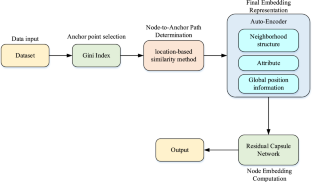
Data Availability
The data supporting the findings of this study are openly available at https://noesis.ikor.org/datasets/link-prediction .
Kumar A, Singh SS, Singh K, Biswas B. Link prediction techniques, applications, and performance: a survey. Physica A. 2020;553: 124289. https://doi.org/10.1016/j.physa.2020.124289 .
Article MathSciNet Google Scholar
Yuliansyah H, Othman ZA, Bakar AA. Taxonomy of link prediction for social network analysis: a review. IEEE Access. 2020;8:183470–87. https://doi.org/10.1109/ACCESS.2020.3029122 .
Article Google Scholar
Rossi A, Barbosa D, Firmani D, Matinata A, Merialdo P. Knowledge graph embedding for link prediction: a comparative analysis. ACM Trans Knowl Discov Data. 2021;15(2):1–49. https://doi.org/10.1145/3424672 .
Zhu Z, Zhang Z, Xhonneux L.P., Tang J. Neural Bellman-Ford networks: a general graph neural network framework for link prediction. In: Ranzato M, Beygelzimer A, Dauphin Y, Liang PS, Vaughan JW, editors. Advances in Neural Information Processing Systems, Curran Associates, Inc., 2021, pp. 29476–29490. [Online]. Available: https://proceedings.neurips.cc/paper_files/paper/2021/file/f6a673f09493afcd8b129a0bcf1cd5bc-Paper.pdf .
Yun S, Kim S, Lee J, Kang J, Kim HJ. Neo-GNNs: neighborhood overlap-aware graph neural networks for link prediction. In: Ranzato M, Beygelzimer A, Dauphin Y, Liang PS, Vaughan JW, editors. Advances in neural information processing systems, Curran Associates, Inc., 2021, pp. 13683–13694. [Online]. Available: https://proceedings.neurips.cc/paper_files/paper/2021/file/71ddb91e8fa0541e426a54e538075a5a-Paper.pdf .
Zhang Z, Cai J, Zhang Y, Wang J. Learning hierarchy-aware knowledge graph embeddings for link prediction. AAAI. 2020;34(03):3065–72. https://doi.org/10.1609/aaai.v34i03.5701 .
Nasiri E, Berahmand K, Li Y. A new link prediction in multiplex networks using topologically biased random walks. Chaos Solitons Fractals. 2021;151: 111230. https://doi.org/10.1016/j.chaos.2021.111230 .
Yang C et al. Few-shot link prediction in dynamic networks. In: Proceedings of the Fifteenth ACM International Conference on Web Search and Data Mining, Virtual Event AZ USA: ACM, Feb. 2022, pp. 1245–1255. https://doi.org/10.1145/3488560.3498417 .
Bai S, Zhang Y, Li L, Shan N, Chen X. Effective link prediction in multiplex networks: a TOPSIS method. Expert Syst Appl. 2021;177: 114973. https://doi.org/10.1016/j.eswa.2021.114973 .
Najari S, Salehi M, Ranjbar V, Jalili M. Link prediction in multiplex networks based on interlayer similarity. Physica A. 2019;536: 120978. https://doi.org/10.1016/j.physa.2019.04.214 .
Quach KG et al. DyGLIP: a dynamic graph model with link prediction for accurate multi-camera multiple object tracking. 2021. https://doi.org/10.48550/ARXIV.2106.06856 .
Li K, Tu L, Chai L. Ensemble-model-based link prediction of complex networks. Comput Netw. 2020;166: 106978. https://doi.org/10.1016/j.comnet.2019.106978 .
Kim J, Geum Y. How to develop data-driven technology roadmaps: The integration of topic modeling and link prediction. Technol Forecast Soc Chang. 2021;171: 120972. https://doi.org/10.1016/j.techfore.2021.120972 .
Lim M, Abdullah A, Jhanjhi N, Supramaniam M. Hidden link prediction in criminal networks using the deep reinforcement learning technique. Computers. 2019;8(1):8. https://doi.org/10.3390/computers8010008 .
Wang G, Wang Y, Li J, Liu K. A multidimensional network link prediction algorithm and its application for predicting social relationships. J Comput Sci. 2021;53: 101358. https://doi.org/10.1016/j.jocs.2021.101358 .
Wahid-Ul-Ashraf A, Budka M, Musial K. How to predict social relationships—physics-inspired approach to link prediction. Physica A. 2019;523:1110–29. https://doi.org/10.1016/j.physa.2019.04.246 .
Stoica G, Stretcu O, Platanios EA, Mitchell T, Póczos B. Contextual parameter generation for knowledge graph link prediction. AAAI. 2020;34(03):3000–8. https://doi.org/10.1609/aaai.v34i03.5693 .
Li S, Song X, Lu H, Zeng L, Shi M, Liu F. Friend recommendation for cross marketing in online brand community based on intelligent attention allocation link prediction algorithm. Expert Syst Appl. 2020;139: 112839. https://doi.org/10.1016/j.eswa.2019.112839 .
Liu G. An ecommerce recommendation algorithm based on link prediction. Alex Eng J. 2022;61(1):905–10. https://doi.org/10.1016/j.aej.2021.04.081 .
Chen H, Yin H, Sun X, Chen T, B. Gabrys B, Musial K. Multi-level graph convolutional networks for cross-platform anchor link prediction. In: Proceedings of the 26th ACM SIGKDD International Conference on knowledge discovery & data mining, Virtual Event CA USA: ACM, Aug. 2020, pp. 1503–1511. https://doi.org/10.1145/3394486.3403201 .
Yi T, Zhang S, Bu Z, Du J, Fang C. Link prediction based on higher-order structure extraction and autoencoder learning in directed networks. Knowl-Based Syst. 2022;241: 108241. https://doi.org/10.1016/j.knosys.2022.108241 .
Liu X, Li X, Fiumara G, De Meo P. Link prediction approach combined graph neural network with capsule network. Expert Syst Appl. 2023;212: 118737. https://doi.org/10.1016/j.eswa.2022.118737 .
Zhang P, Chen J, Che C, Zhang L, Jin B, Zhu Y. IEA-GNN: Anchor-aware graph neural network fused with information entropy for node classification and link prediction. Inf Sci. 2023;634:665–76. https://doi.org/10.1016/j.ins.2023.03.022 .
Chen J, Wang X, Xu X. GC-LSTM: graph convolution embedded LSTM for dynamic network link prediction. Appl Intell. 2022;52(7):7513–28. https://doi.org/10.1007/s10489-021-02518-9 .
Zeb A, Saif S, Chen J, Haq AU, Gong Z, Zhang D. Complex graph convolutional network for link prediction in knowledge graphs. Expert Syst Appl. 2022;200: 116796. https://doi.org/10.1016/j.eswa.2022.116796 .
Dong L, Yao H, Li D, Wang Y, Li S, Liang Q. Improving graph neural network via complex-network-based anchor structure. Knowl-Based Syst. 2021;233: 107528. https://doi.org/10.1016/j.knosys.2021.107528 .
Liu Z, Fang Y, Liu Y, Zheng VW. Neighbor-anchoring adversarial graph neural networks. IEEE Trans Knowl Data Eng. 2021. https://doi.org/10.1109/TKDE.2021.3087970 .
Ceriani L, Verme P. The origins of the Gini index: extracts from Variabilità e Mutabilità (1912) by Corrado Gini. J Econ Inequal. 2012;10(3):421–43. https://doi.org/10.1007/s10888-011-9188-x .
Zhi T, Luo H, Liu Y. A Gini impurity-based interest flooding attack defence mechanism in NDN. IEEE Commun Lett. 2018;22(3):538–41. https://doi.org/10.1109/LCOMM.2018.2789896 .
noesis. [Online]. Available: https://noesis.ikor.org/datasets/link-prediction .
Watts DJ, Strogatz SH. Collective dynamics of ‘small-world’ networks. Nature. 1998;393(6684):440–2. https://doi.org/10.1038/30918 .
Guimerà R, Danon L, Díaz-Guilera A, Giralt F, Arenas A. Self-similar community structure in a network of human interactions. Phys Rev E. 2003;68(6): 065103. https://doi.org/10.1103/PhysRevE.68.065103 .
Batagelj V, Mrvar A. Pajek datasets. 2006. [Online]. Available: http://vlado.fmf.uni-lj.si/pub/networks/data/ .
Massa P, Salvetti M, Tomasoni D. Bowling alone and trust decline in social network sites. In: 2009 Eighth IEEE International Conference on Dependable, Autonomic and Secure Computing, Chengdu, China: IEEE, Dec. 2009, pp. 658–663. https://doi.org/10.1109/DASC.2009.130 .
“PGP Dataset.” [Online]. Available: http://konect.cc/networks/arenas-pgp/ .
Serrano MÁ, Boguñá M, Pastor-Satorras R, Vespignani A. Correlations in complex networks. In: Complex Systems and Interdisciplinary Science, vol. 2, WORLD SCIENTIFIC, 2007, pp. 35–65. https://doi.org/10.1142/9789812771681_0004 .
Bu D. Topological structure analysis of the protein-protein interaction network in budding yeast. Nucleic Acids Res. 2003;31(9):2443–50. https://doi.org/10.1093/nar/gkg340 .
Peri S, et al. Development of human protein reference database as an initial platform for approaching systems biology in humans. Genome Res. 2003;13(10):2363–71. https://doi.org/10.1101/gr.1680803 .
Political books. 2004. [Online]. Available: http://konect.cc/networks/dimacs10-polbooks/ .
Leskovec J, Mcauley J. Learning to discover social circles in ego networks. In: Advances in neural information processing systems, F. Pereira, C. J. Burges, L. Bottou, and K. Q. Weinberger, Eds., Curran Associates, Inc., 2012. [Online]. Available: https://proceedings.neurips.cc/paper_files/paper/2012/file/7a614fd06c325499f1680b9896beedeb-Paper.pdf .
Newman MEJ. The structure of scientific collaboration networks. Proc Natl Acad Sci USA. 2001;98(2):404–9. https://doi.org/10.1073/pnas.98.2.404 .
Isella L, Stehlé J, Barrat A, Cattuto C, Pinton J-F, den Broeck WV. What’s in a crowd? Analysis of face-to-face behavioral networks. 2010. https://doi.org/10.48550/ARXIV.1006.1260 .
Newman MEJ. Finding community structure in networks using the eigenvectors of matrices. Phys Rev E. 2006;74(3): 036104. https://doi.org/10.1103/PhysRevE.74.036104 .
“Hamsterster.” [Online]. Available: http://konect.cc/networks/petster-hamster/ . Accessed Dec 2023.
Xu Z, Harriss R. Exploring the structure of the US intercity passenger air transportation network: a weighted complex network approach. GeoJournal. 2008;73(2):87. https://doi.org/10.1007/s10708-008-9173-5 .
Leskovec J, Kleinberg J, Faloutsos C. Graph evolution: densification and shrinking diameters. ACM Trans Knowl Discov Data. 2007;1(1):2. https://doi.org/10.1145/1217299.1217301 .
Download references
The authors did not receive support from any organization for the submitted work. No funding was received to assist with the preparation of this manuscript. No funding was received for conducting this study. No funds, grants, or other support was received.
Author information
Authors and affiliations.
Computer Science & Engineering and IT, Jaypee Institute of Information Technology, Noida, India
Shambhu Kumar & Arti Jain
Department of Mathematics, Jaypee Institute of Information Technology, Noida, India
Dinesh Bisht
You can also search for this author in PubMed Google Scholar
Contributions
Shambhu Kumar: Methodology, Software, Writing- Original draft preparation, Investigation. Arti Jain.: Conceptualization, Supervision, Writing- Reviewing and Editing. Dinesh C. S. Bisht: Visualization, Supervision, Writing- Reviewing and Editing.
Corresponding author
Correspondence to Arti Jain .
Ethics declarations
Conflict of interest.
The authors declare that they have no competing financial or non-financial interests. The authors have no conflicts of interest to declare that they are relevant to the content of this article. All authors certify that they have no affiliations with or involvement in any organization or entity with any financial interest or non-financial interest in the subject matter or materials discussed in this manuscript. The authors have no financial or proprietary interests in any material discussed in this article.
Research Involving Human and/or Animals
The study solely relied on computational methods and utilized pre-existing datasets, thereby excluding the involvement of human or animal subjects. Consequently, ethical approval or informed consent was not deemed necessary.
Informed Consent
Informed consent was obtained from all individual participants included in the study.
Additional information
Publisher's note.
Springer Nature remains neutral with regard to jurisdictional claims in published maps and institutional affiliations.
Rights and permissions
Springer Nature or its licensor (e.g. a society or other partner) holds exclusive rights to this article under a publishing agreement with the author(s) or other rightsholder(s); author self-archiving of the accepted manuscript version of this article is solely governed by the terms of such publishing agreement and applicable law.
Reprints and permissions
About this article
Kumar, S., Bisht, D. & Jain, A. An Anchor-Aware Graph Autoencoder Fused with Gini Index Model for Link Prediction. SN COMPUT. SCI. 5 , 745 (2024). https://doi.org/10.1007/s42979-024-03081-z
Download citation
Received : 25 January 2024
Accepted : 20 June 2024
Published : 31 July 2024
DOI : https://doi.org/10.1007/s42979-024-03081-z
Share this article
Anyone you share the following link with will be able to read this content:
Sorry, a shareable link is not currently available for this article.
Provided by the Springer Nature SharedIt content-sharing initiative
- Ideal Anchor Point
- Path Estimation Portion
- Path information function
- Link prediction
- Capsule network
- Residual module
- Shortest path distance
- Find a journal
- Publish with us
- Track your research
IMAGES
VIDEO
COMMENTS
CSC 170 - Introduction to Computers and Their Applications Lecture #1 - Digital Basics Data Representation • Data refers to the symbols that represent people, events, things, and ideas. Data can be a name, a number, the colors in a photograph, or the notes in a musical composition. • Data Representation refers to the form in which
The operating system and hardware ensure that data in this segment is not changed during the lifetime of the program. Any attempt to modify data in the code segment will cause a crash. i1, the int global object, has the next highest address. It is in the data segment, which holds modifiable global data. This segment keeps the same size as the ...
A computer uses a fixed number of bits to represent a piece of data which could be a number, a character, image, sound, video, etc. Data representation is the method used internally to represent data in a computer. Let us see how various types of data can be represented in computer memory. Before discussing data representation of numbers, let ...
Introduction to Computer Data Representation introduces readers to the representation of data within computers. Starting from basic principles of number representation in computers, the book covers the representation of both integer and floating point numbers, and characters or text. It comprehensively explains the main techniques of computer arithmetic and logical manipulation.
Data Representation. Data Representation. Eric Roberts. CS 106A February 10, 2016. Structure of MemoryThe fundamental unit of memory inside a computer is called a bit, which is a contraction of the. ords binary digit. A bit can be in either of two states, usually. enoted as 0 and 1.The hardware structure of a computer combines individual bit.
Introduction to Computer Data Representation also includes historical aspects of data representation, explaining some of the steps that developers took (and the mistakes they made) that led to the present, well-defined and accepted standards of data representation techniques. The book serves as a primer for advanced computer science graduates ...
Introduction to Computer Data Representation also includes historical aspects of data representation, explaining some of the steps that developers took (and the mistakes they made) that led to the present, well-defined and accepted standards of data representation techniques. The book serves as a primer for advanced computer science graduates ...
Introduction to Computer Data Representation also includes historical aspects of data representation, explaining some of the steps that developers took (and the mistakes they made) that led to the present, well-defined and accepted standards of data representation techniques. The book serves as a primer for advanced computer science graduates ...
The problem of data representation is the problem of representing all the concepts we might want to use in programming—integers, fractions, real numbers, sets, pictures, texts, buildings, animal species, relationships—using the limited medium of addresses and bytes. Powers of ten and powers of two.
An 8-bit code, used now only by some IBM mainframes. UNICODE. Provides a unique number for every character. A family of encodings - 8, 16, and 32 bits per character. Allows a greater variety of characters. Able to represent virtually any character in use today in any language, and some no longer in use.
Mantissa, Significand and fraction are synonymously used terms. In the computer, the representation is binary and the binary point is not fixed. For example, a number, say, 23.345 can be written as 2.3345 x 101 or 0.23345 x 10² or 2334.5 x 10-2. The representation 2.3345 x 101 is said to be in normalised form.
For the computer to be able to manipulate any data or information from whatever source, or act on any instruction, that data, information or instructions mus...
Introduction to Computer Data Representation also includes historical aspects of data representation, explaining some of the steps that developers took (and the mistakes they made) that led to the present, well-defined and accepted standards of data representation techniques. The book serves as a primer for advanced computer science graduates ...
Data Representation in Digital Computers Dr. McCloskey Introduction. To introduce this subject, let us consider an example that may help you to understand more clearly the idea of representing one thing by another. Take the word cat. It refers to a class of animals, often kept as pets by humans, whose members have certain common characteristics ...
When we look at a computer, we see text and images and shapes. To a computer, all of that is just binary data, 1s and 0s. The following 1s and 0s represents a tiny GIF: This next string of 1s and 0s represents a command to add a number: You might be scratching your head at this point. Why do computers represent information in such a hard to ...
Data Representation Techniques. Classification of Computers. Computer scans are classified broadly based on their speed and computing power. 1. Microcomputers or PCs (Personal Computers): It is a single-user computer system with a medium-power microprocessor. It is referred to as a computer with a microprocessor as its central processing unit.
Introduction to Computer Data Representation also includes historical aspects of data representation, explaining some of the steps that developers took (and the mistakes they made) that led to the present, well-defined and accepted standards of data representation techniques. The book serves as a primer for advanced computer science graduates ...
Title: Introduction to Computer Data Representation Author: Fenwick, Peter(Author) Created Date: 4/4/2014 12:31:59 PM
Introduction to Computer Data Representation 1st Edition is written by Peter Fenwick and published by Bentham Science. The Digital and eTextbook ISBNs for Introduction to Computer Data Representation are 9781608058822, 1608058824 and the print ISBNs are 9781608058839, 1608058832. Save up to 80% versus print by going digital with VitalSource.
Introduction to Computer Data Representation introduces readers to the representation of data within computers. Starting from basic principles of number representation in computers, the book covers the representation of both integer and floating p...
Representation of Data/Information - Computers do not understand human language; they understand data within the prescribed form. Data representation is a method to represent data and encode it in a computer system. Generally, a user inputs numbers, text, images, audio, and video etc types of data to process but the computer converts t.
The terms bits, bytes, nibble and word are used widely in reference to computer memory and data size. Bits: can be defined as either a binary, which can be 0, or 1.It is the basic unit of data or information in digital computers. Byte: a group of bits (8 bits) used to represent a character.
Contrastive Language Image Pre-training (CLIP) has recently demonstrated success across various tasks due to superior feature representation empowered by image-text contrastive learning. However, the instance discrimination method used by CLIP can hardly encode the semantic structure of training data. To handle this limitation, cluster discrimination has been proposed through iterative cluster ...
Previous deepfake detection methods mostly depend on low-level textural features vulnerable to perturbations and fall short of detecting unseen forgery methods. In contrast, high-level semantic features are less susceptible to perturbations and not limited to forgery-specific artifacts, thus having stronger generalization. Motivated by this, we propose a detection method that utilizes high ...
Link prediction stands as a crucial network challenge, garnering attention over the past decade, with its significance heightened by the escalating volume of network data. In response to the pressing need for swift research focus, this study introduces an innovative approach—the Anchor-aware Graph Autoencoder integrated with the Gini Index (AGA-GI)—aimed at gathering data on the global ...
The data processing and pooling for this study were done using either MATLAB 2020a 124,125 and/or Microsoft Excel (2020). 139 All the graphs and statistical analysis were derived using GraphPad Prism software version 9.1.0 for Windows (GraphPad Software, San Diego, CA, USA). 140 The normality of the data distribution for all the variables was ...