Well Logging: Principles, Applications and Uncertainties
- January 2015
- In book: Petroleum Geoscience-From Sedimentary Environments to Rock Physics
- Edition: Second Edition
- Chapter: 16
- Publisher: Springer-Verlag Berlin Heidelber
- Editors: Knut Bjørlykke

- University of Oslo

Abstract and Figures

Discover the world's research
- 25+ million members
- 160+ million publication pages
- 2.3+ billion citations
- Geotech Geol Eng

- Júlio de Castro Vargas Fernandes
- Carlos E. M. dos Anjos

- Hiroki Tanaka

- Ammar Qatari

- MAR PETROL GEOL

- George Coates
- Manfred Prammer
- A. Guy Plint
- W.S. Donaldson
- Jens Jahren

- G.B. ASQUITH
- Daniel Krygowski
- Q.R. Passey
- F. J. Moretti
- J. B. Kulla
- J. D. Stroud
- A. C. Dumestre

- Recruit researchers
- Join for free
- Login Email Tip: Most researchers use their institutional email address as their ResearchGate login Password Forgot password? Keep me logged in Log in or Continue with Google Welcome back! Please log in. Email · Hint Tip: Most researchers use their institutional email address as their ResearchGate login Password Forgot password? Keep me logged in Log in or Continue with Google No account? Sign up
Information
- Author Services
Initiatives
You are accessing a machine-readable page. In order to be human-readable, please install an RSS reader.
All articles published by MDPI are made immediately available worldwide under an open access license. No special permission is required to reuse all or part of the article published by MDPI, including figures and tables. For articles published under an open access Creative Common CC BY license, any part of the article may be reused without permission provided that the original article is clearly cited. For more information, please refer to https://www.mdpi.com/openaccess .
Feature papers represent the most advanced research with significant potential for high impact in the field. A Feature Paper should be a substantial original Article that involves several techniques or approaches, provides an outlook for future research directions and describes possible research applications.
Feature papers are submitted upon individual invitation or recommendation by the scientific editors and must receive positive feedback from the reviewers.
Editor’s Choice articles are based on recommendations by the scientific editors of MDPI journals from around the world. Editors select a small number of articles recently published in the journal that they believe will be particularly interesting to readers, or important in the respective research area. The aim is to provide a snapshot of some of the most exciting work published in the various research areas of the journal.
Original Submission Date Received: .
- Active Journals
- Find a Journal
- Proceedings Series
- For Authors
- For Reviewers
- For Editors
- For Librarians
- For Publishers
- For Societies
- For Conference Organizers
- Open Access Policy
- Institutional Open Access Program
- Special Issues Guidelines
- Editorial Process
- Research and Publication Ethics
- Article Processing Charges
- Testimonials
- Preprints.org
- SciProfiles
- Encyclopedia
Journal Menu
- Processes Home
- Aims & Scope
- Editorial Board
- Reviewer Board
- Topical Advisory Panel
- Instructions for Authors
- Special Issues
- Sections & Collections
- Article Processing Charge
- Indexing & Archiving
- Editor’s Choice Articles
- Most Cited & Viewed
- Journal Statistics
- Journal History
- Journal Awards
- Society Collaborations
- Conferences
- Editorial Office
Journal Browser
- arrow_forward_ios Forthcoming issue arrow_forward_ios Current issue
- Vol. 12 (2024)
- Vol. 11 (2023)
- Vol. 10 (2022)
- Vol. 9 (2021)
- Vol. 8 (2020)
- Vol. 7 (2019)
- Vol. 6 (2018)
- Vol. 5 (2017)
- Vol. 4 (2016)
- Vol. 3 (2015)
- Vol. 2 (2014)
- Vol. 1 (2013)
Find support for a specific problem in the support section of our website.
Please let us know what you think of our products and services.
Visit our dedicated information section to learn more about MDPI.
Rock Physics, Well Logging, and Formation Evaluation in Energy Exploration Systems
- Print Special Issue Flyer
Special Issue Editors
Special issue information, benefits of publishing in a special issue.
- Published Papers
A special issue of Processes (ISSN 2227-9717). This special issue belongs to the section " Energy Systems ".
Deadline for manuscript submissions: 10 December 2024 | Viewed by 29471
Share This Special Issue

Dear Colleagues,
Well logging plays a very important role in oil and gas exploration and development since it appeared in 1927. It can help to indicate effective formations, offer reliable formation parameters and identify fluids. In the last decade, as more and more unconventional oil and gas, e.g., shale oil/gas and tight oil/gas, are discovered, common well logging inversion and interpretation techniques face great challenges. Formation evaluation methods also cannot work. For complex reservoir characterization, validity evaluation and “sweet spot” prediction, it is urgent to put forward innovative evaluation methods. In addition, small pore space, poor connectivity and weak fluid response lead to low formation parameter (especially permeability and water saturation) calculation and hydrocarbon-beariong identification accuracy. The emergence of digital rock physics techniques and deep learning methods provides a new direction to solve the problem of complex formation evaluation.
This Special Issue on ‘Rock Physics, Well Logging, and Formation Evaluation in Energy Exploration Systems’ seeks high-quality works focusing on the latest novel advances for conventional and unconventional reservoir evaluation based on rock physics and well logging. Topics include, but are not limited to:
- Conventional and unconventional reservoir characterization based on well logging techniques;
- Shale oil/gas, tight oil/gas identification and “sweet spot” prediction;
- Unconventional reservoir conduction mechanism and parameter evaluation;
- Application of deep learning methods in formation evaluation;
- Digital rock physics or NMR techniques for complex formation evaluation.
Prof. Dr. Liang Xiao Dr. Xin Nie Prof. Dr. Mehdi Ostadhassan Dr. Hongyan Yu Guest Editors
Manuscripts should be submitted online at www.mdpi.com by registering and logging in to this website . Once you are registered, click here to go to the submission form . Manuscripts can be submitted until the deadline. All submissions that pass pre-check are peer-reviewed. Accepted papers will be published continuously in the journal (as soon as accepted) and will be listed together on the special issue website. Research articles, review articles as well as short communications are invited. For planned papers, a title and short abstract (about 100 words) can be sent to the Editorial Office for announcement on this website.
Submitted manuscripts should not have been published previously, nor be under consideration for publication elsewhere (except conference proceedings papers). All manuscripts are thoroughly refereed through a single-blind peer-review process. A guide for authors and other relevant information for submission of manuscripts is available on the Instructions for Authors page. Processes is an international peer-reviewed open access monthly journal published by MDPI.
Please visit the Instructions for Authors page before submitting a manuscript. The Article Processing Charge (APC) for publication in this open access journal is 2400 CHF (Swiss Francs). Submitted papers should be well formatted and use good English. Authors may use MDPI's English editing service prior to publication or during author revisions.
- formation evaluation
- pore structure
- validity characterization
- deep learning
- digital rock physics
- Ease of navigation: Grouping papers by topic helps scholars navigate broad scope journals more efficiently.
- Greater discoverability: Special Issues support the reach and impact of scientific research. Articles in Special Issues are more discoverable and cited more frequently.
- Expansion of research network: Special Issues facilitate connections among authors, fostering scientific collaborations.
- External promotion: Articles in Special Issues are often promoted through the journal's social media, increasing their visibility.
- e-Book format: Special Issues with more than 10 articles can be published as dedicated e-books, ensuring wide and rapid dissemination.
Further information on MDPI's Special Issue polices can be found here .
Published Papers (22 papers)
Further Information
Mdpi initiatives, follow mdpi.
Subscribe to receive issue release notifications and newsletters from MDPI journals
ORIGINAL RESEARCH article
Digital construction of geophysical well logging curves using the lstm deep-learning network.

- College of Geophysics and Petroleum Resources, Yangtze University, Wuhan, China
A complete well logging suite is needed frequently, but it is either unavailable or has missing parts. The mudstone section is prone to wellbore collapse, which often causes distortion in well logs. In many cases, well logging curves are never measured, yet are needed for petrophysical or other analyses. Re-logging is expensive and difficult to achieve, while manual construction of the missing well logging curves is costly and low in accuracy. The rapid technical evolution of deep-learning algorithms makes it possible to realize the digital construction of missing well logging curves with high precision in an automated fashion. In this article, a workflow is proposed for the digital construction of well logging curves based on the long short-term memory (LSTM) network. The LSTM network is chosen because it has the advantage of avoiding the vanishing gradient problem that exists in traditional recurrent neural networks (RNNs). Additionally, it can process sequential data. When it is used in the construction of missing well logging curves, it not only considers the relationship between each logging curve but also the influence of the data from a previous depth on data at the following depth. This influence is validated by exercises constructing acoustic, neutron porosity, and resistivity logging curves using the LSTM network, which effectively achieves high-precision construction of these missing curves. These exercises show that the LSTM network is highly superior to the RNN in the digital construction of well logging curves, in terms of accuracy, efficiency, and reliability.
Introduction
During well logging operations, borehole damage or collapse occurs frequently in the mudstone section, resulting in distortion in well logs, and even more seriously, in missing well logging curves. Instrument failure and logging environments can also lead to lost or erroneous logging curves. In petrophysical analysis, a comprehensive analysis of all the depths of the well logging curves is usually a must. As a result, the distortion or absence of a particular section of the logging curve will have profound reverse effects on the results of the final analysis. Therefore, it is necessary for the entire logging curve to be reliable with high accuracy, for which an efficient, simple, and accurate logging curve construction method is particularly essential.
Re-logging can be used to obtain the missing logging curves. However, doing so will significantly increase the cost from the standpoint of both labor and equipment. Moreover, re-logged curves may deviate from those in the original logging environment due to changes in that environment, for example, mud-filtrate invasion. Many other methods for reconstructing the missing logging curves have been investigated in the literature, such as empirical formulas, correlation correction methods, forward modeling correction methods, and multi-variate regression methods ( Zhang et al., 2018 ; Zhou et al., 2021 ). If the borehole collapses and the logging curve distortion is serious, the correlation correction method will not succeed. The forward modeling correction method requires accurate knowledge of the complex physical properties ( Asquith et al., 2004 ; Bateman, 2012 ), which are not readily available. Although those methods can reconstruct the missing logging curve to a certain extent, they ignore the complexity and strong non-uniformity of the formation conditions, thus greatly simplifying the real formation conditions, and hindering the predicted results from meeting the accuracy requirements of logging interpretation and reservoir characterization ( Bassiouni, 1994 ).
With the advancement of computer and information technology, machine learning has become a powerful tool for model construction and prediction ( Ramaswamy et al., 2000 ; Cawley 2006 ; Kusiak et al., 2010 ; Marvuglia and Messineo, 2012 ; Hu et al., 2014 ), and has undoubtedly found applications in the field of petroleum exploration and production ( Iturrar N-Viveros and Parra, 2014 ; Zerrouki et al., 2014 ; Chen 2020 ). Potential machine-learning algorithms include support vector machines (SVMs), artificial neural networks (ANNs), recurrent neural networks (RNNs), and generative adversarial networks (GANs) ( Goodfellow et al., 2014 ; Goodfellow, 2016 ). Rolon et al. (2009) used the generalized regression neural network to reconstruct the missing logging curves, and the experimental results show that synthetic logging curves from the neural network are more accurate than those from traditional multi-variate regression, linear regression, and other methods ( Rolon et al., 2009 ). Salehi et al. (2017) reconstructed density and electrical logs using the multilayer perceptron (MLP). Yang et al. (2008) used the back propagation (BP) neural network to reconstruct acoustic logging curves, and verified that the method could significantly improve the quality of acoustic logging curves affected by wellbore collapse. Hu (2020) adopted the GAN with constraint conditions to learn the distribution of real logging curves, and introduced the mean square error into the objective function of the original GAN to improve the learning ability of the model. He demonstrated that, compared with the Kriging interpolation method and the fully connected neural network, this method performs better in predicting the logging curve. However, although the above methods are able to reconstruct the missing well logging curves to a certain extent, it is still difficult to achieve high accuracy.
In this article, we demonstrate that the LSTM network is a deep-learning algorithm naturally suited to the digital reconstruction of well logging curves. This is because the well logging curve has the characteristic of a time sequence, due to the connection of the curve from point to point. When dealing with these kinds of data, we should not only consider the interaction between each well logging curve, but also the influence of the previous data point on the following data point. Recurrent neural networks (RNNs) are very effective in processing data with sequential characteristics ( Schuster and Paliwal, 1997 ). However, a regular RNN has the problem of a vanishing gradient, which effectively prevents the weight in the neural network from changing its value and hence stops the neural network from further training.
The long short-term memory (LSTM) network ( Hochreiter and Schmidhuber, 1997 ) is a variant of the RNN. Compared with the RNN, the LSTM network has three more control devices: input control, forget control, and output control, which can better retain the required data. The LSTM network overcomes the problem of the vanishing gradient that exists in the RNN, making it more effective and reliable for training the well logging curves. It has found application in many different domains. Zhao et al. (2021) developed a hybrid model by combining a long short-term memory network (LSTM), a convolutional neural network (CNN), and a singular spectrum analysis (SSA). Among these, the LSTM network effectively extracted the time features, and the hybrid model could accurately extract data features of monitoring signals and further improve the recognition performance of mass spectral signals. Thus, the long short-term memory network has significant advantages in processing time-series data. Shashidhar et al. (2022) adopted the LSTM method for visual speech recognition, and the research results show that this network can recognize speech very well. Ma et al. (2022) applied LSTM to predicting the normal passenger flow and emergency passenger flow of a metro traffic system. Compared with the traditional data of incoming and outgoing warehouse or IC cards, this method better reflects the passenger flow data of the metro traffic system’s capacity. Absar et al. (2022) used the LSTM model to predict infectious diseases, and their study showed that the algorithm achieved good results in time-series prediction, and could hence effectively reduce infection rates to a certain extent.
In this study, the LSTM method is used to reconstruct the missing logging curves through the TensorFlow ( Martín et al., 2016 ) framework, and the reliability of the model is verified using field well logs. Experimental studies show that, compared to the RNN, the LSTM network is very efficient, accurate, and concise for the generation of digital well logging curves.
Methodology
Correlation analysis.
Correlation analysis refers to the analysis of the degree of correlation between two or more variables. In this work, it is necessary to perform correlation analysis and find the logging curves that have the highest correlation with the target logging curve. The existence of some correlation is necessary to predict one variable from another. Pearson’s ( 1920 ) correlation coefficient is used to in this work. Assuming that there are two variables, X and Y , Pearson’s correlation coefficient between X and Y can be expressed as follows:
where E represents the mathematical expectation and cov(X, Y) represents the covariance between variable X and variable Y ; μ X , μ y are the mean for variable X and variable Y , respectively; and σ X , σ Y are the standard deviation for variable X and variable Y , respectively. The value range of Pearson’s coefficient p is [-1,1]. The positive and negative values of the p -value represent the direction of correlation, and the magnitude of its absolute value represents the degree of correlation. When the p -value is greater than 0, X and Y are positively correlated, and the greater the p -value, the higher the correlation. By contrast, if the p -value is less than 0, X and Y are negatively correlated; if the p -value is 0, there is no linear relationship between X and Y ; and if the absolute value of p is 1, X and Y are completely linearly correlated. A rule of thumb for measuring the significance of the correlation is as follows: 0.0 < | p | < 0.2 means very weakly related or unrelated, 0.2 < | p | < 0.4 means a weak correlation, 0.4 < | p | < 0.6 means moderately related, 0.6 < | p | < 0.8 means a strong correlation, and 0.8 < | p | < 1.0 means a very strong correlation.
Data normalization
The purpose of data normalization is to map large data or small data in a data set to the same range. The most common range is (0, 1), which is convenient for subsequent data processing and model training. The maximum and minimum normalization is adopted in this study, and its formula is shown as follows:
where x is the data sample and x max and x min are the maximum and minimum values in the x sample, respectively. Using Eq. 2 , all the data samples can be mapped to between 0 and 1.
The recurrent neural network
The recurrent neural network ( Chung et al., 2015 ) is a kind of recursive neural network that takes sequence data as input, and recurses in the evolutionary direction of sequence where all nodes (cyclic units) are linked by chain. The RNN is very effective for processing sequential data, which are arranged in a certain chronological or logical order. The RNN simply consists of an input layer, a hidden layer, and an output layer, which is shown below.
Figure 1 is the basic structure of an RNN. It does not show all the nodes of the recurrent neural network. Assuming that the arrow above W is removed, this network becomes the most common fully connected neural network. The X vector represents the input layer data, S represents the value of the hidden layer, and the O vector represents the value of the output layer. It should be noted that in actual problems, the input layer, output layer, and hidden layer are not one node as shown in the figure above; instead, each layer actually contains multiple nodes. Here U is the weight from the input layer to the hidden layer, V is the weight from the hidden layer to the output layer, and W is the weight of the last hidden layer as the input for this time. It can therefore be seen that the hidden layer of the recurrent neural network is composed of the current input value X and the last hidden value S. An expanded recurrent neural network is shown below. The related formulas are as follows:

FIGURE 1 . Basic structure of the recurrent neural network.
Figure 2 is the expansion of Figure 1 . It can be seen from Figure 2 or Eq. 4 that the received value at time t in this network consists of the input X t and the output of a hidden layer at a previous time, which reveals how the recurrent neural network works. It can be seen from Eqs 3 , 4 that the specific calculation process of the recurrent neural network is obtained by multiplying the input by the corresponding weight before finally adding the activation function. Throughout the training process, the same weight W is used for each moment. A cyclic neural network is similar to a multilayer neural network: as the number of neurons increases, the RNN also has the problems of gradient explosion and gradient disappearance in the process of back propagation ( Franke et al., 2012 ).

FIGURE 2 . Expanded structure of the recurrent neural network.
The LSTM network
In order to eliminate the problems of gradient explosion, gradient disappearance etc., various improved recurrent neural networks have been proposed instead of the traditional RNNs. The long short-term memory network is a variant of the recurrent neural network. The recurrent neural network will store all the values of the hidden layer at each moment and apply them to the next moment, thus ensuring that each moment contains the information of the previous moment. The LSTM network selectively stores information by adding three gating devices, namely input control, output control, and forget control, compared with the hidden layer that stores all data in the recurrent neural network. The LSTM is composed of a series of recursively connected sub-networks of memory blocks, each of which contains one or more memory cells and three multiplication units (input gate, output gate, and forget gate), which can carry out continuous write, read, and reset operations on memory cells ( Hochreiter and Schmidhuber, 1997 ; Graves et al., 2013 ). The LSTM can thus effectively mitigate the problems of gradient disappearance and gradient explosion that exist in the traditional RNN ( Cho et al., 2014 ). The internal structure of the LSTM network is shown in Figure 3 . Excluding the nodes in each neural unit, an LSTM network is an RNN.

FIGURE 3 . Structure of the LSTM network.
Firstly, the forget gate determines how much information in the unit state C t-1 of the previous moment will be retained in the current moment C t . The input X t of the current moment is combined with the hidden state of the previous moment to form a new vector, and is then multiplied by the weight coefficient W, and finally through the sigmoid function. The result is multiplied by the unit state C t-1 at the last moment to determine how much information is added to the unit state C t-1 at the last moment. The expression of the forget gate control for this time is
Secondly, the input gate controls how much information from the input X t of the current moment will be retained in the cell state C t of the current moment. The sigmoid function determines which values need to be updated for the input gate layer. The tanh function determines the candidate value C ∼ t at the current time and is multiplied by the current i t vector to finally determine how much of the candidate information is input into the cell state C t , where the expression is
Finally, the output gate controls how much state C of the unit is output to the hidden state of the unit. The output gate and output signal are multiplied to determine the amount of information to be output at this moment. The expressions for decision vector O t and the hidden state h t of the cell unit are as follows:
The cell state exists in the whole process, and its function is to update the cell state, that is, to update C t-1 to C, multiply the old state by f t , discard unwanted information, add new candidate values, and determine the change of each cell state according to the result. The formula is as follows:
In the above expressions, X t is the input data of the long short-term memory network at time t ; h t is the data output at time t ; i t , O t , and f t are the activation vector values of input gate, output gate, and forget gate of the LSTM neural network at time t of a node; W f , W i , W c , and W o are the corresponding weights of each structure, respectively; and b i , b c , and b o are the offsets corresponding to each structure, respectively. C is the state of neuron cells, σ is sigmoid function, and tanh is a hyperbolic tangent function.
Comparison of LSTM and RNN
Table 1 lists the comparison of the LSTM network and the RNN. The main advantage of the LSTM network is that it solves the problems of disappearing gradients in RNN, and is more suitable for processing long-memory time-series data.

TABLE 1 . Comparison of LSTM and RNN.
The optimization algorithms
Optimization algorithms are required in the model to update training and output parameters so that they approach or reach the optimum, thereby maximizing (or minimizing) the loss function ( Kingma and Ba, 2015 ). Optimization algorithms are divided into three categories ( Qing, 1999 ). The first category is gradient descent, which includes batch gradient descent, random gradient descent, and small batch gradient descent. These optimization algorithms optimize the model by minimizing the loss function. The second category is momentum optimization methods, including the momentum gradient descent method and the Nesterov accelerated gradient method (NAG). The last category is the adaptive learning rate optimization algorithm, including the AdaGrad, RMSProp, Adam, and AdaDelta methods ( Kingma and Ba, 2015 ). Of these, the Adam (adaptive momentum) optimization algorithm is adopted in this study. This method can calculate the adaptive learning rate for each parameter. The flow chart for the Adam algorithm is shown in Figure 4 .

FIGURE 4 . Flow chart for the Adam optimization algorithm.
In Figure 4 , a is the learning rate, ß 1 , ß 2 ⊂ [0,1) are to control the moving average index attenuation rate; f (θ) is the objective function; θ 0 is the vector for the initial parameter; m 0 is the initial first moment for the gradient (expectation); m 1 is the initial second moment for the gradient (expectation of the square of the gradient); m ^ t and v ^ t are the bias-corrected estimates; t is the time step; and e is a small number. We need to determine the objective function f (θ) and α, β 1 , and β 2 . Here a is generally 0.001, β 1 is 0.9, β 2 is 0.999, and e is 10 −8 . Meanwhile, we need to initialize the parameter vectors θ 0 , the first-order moment vector m t , the second-order moment vector v t , and the time step t . Then we need to determine whether the current θ t converges to less than e . If not, we update each part iteratively; that is, we update t to t+1, the gradient of parameter θ t , the first order matrix m t , and the second-order matrix v t . Then we calculate the first order matrix estimation and the second-order matrix estimation. Finally, we update the parameter θ t . Once the last θ t value is less than ε, the iteration ends and the optimal θ t value is found.
The Adam algorithm is different from the traditional stochastic gradient descent algorithm, which uses a single learning rate to update the weight, and the learning rate does not change in the training process. The Adam algorithm iteratively updates neural network weights based on training data. The Adam algorithm designs different adaptive learning rates for different parameters by calculating the first-order and second-order moment estimation of the gradient, which is the combination of two stochastic gradient descent methods. The adaptive gradient algorithm (AdaGrad) preserves a learning rate for each parameter to improve the performance of sparse gradients in natural language processing and computer vision. Root mean square propagation (RMSProp) adaptively preserves the learning rate for each parameter based on the mean of the nearest magnitude of the weight gradient, which means that the algorithm has good performance on unsteady and on-line problems. The Adam algorithm combines the advantages of the above two algorithms ( Qing, 1999 ). It has the advantages of efficient computation, small memory consumption, and invariable gradient diagonal scaling. It is suitable for solving large-scale optimization problems with big data and parameters, as well as problems of high noise or sparse gradient, and has the advantage of an intuitive interpretation of hyperparameters.
Regularization
Regularization is a general term for a class of methods that add extra terms to loss functions in machine learning to prevent overfitting and to improve model performance. Common regularizations are l 1 regularization and l 2 regularization, or l 1 norm and l 2 norm. The model using l 1 regularization is called lasso regression, and the model using l 2 regularization is called ridge regression. The linear regression l 1 regularization loss function is
while the l 2 regularization loss function is
In Eqs 11 , 12 , ω represents the coefficient of a feature, and the regularization term puts a limit on the coefficient. Here l 1 is regularized as the sum of the absolute values of the elements in the weight vector w , and l 2 is regularized as the sum of squares of the elements in the weight vector w . The regularization term is preceded by a coefficient λ, whose value determines the relative importance of the two terms in Eq. 12 . In order to prevent overfitting in this work, l 2 regularization is used to constrain weight and bias.
Experiments and results analysis
The field well logs used in this study are from X field, including 13 logging curves, namely, computed gamma ray (CGR), uranium (URAN), potassium (POTA), thorium (THOR), shallow lateral resistivity (LLS), deep lateral resistivity (LLD), spontaneous potential (SP), natural gamma ray (GR), borehole diameter (CALI), photoelectric factor (PEF), neutron porosity (NPHI), density (RHOB), and sonic interval transit time (DTCO). There are two natural gamma ray logs: CGR and GR, of which GR is from conventional GR logging, while CGR is from GR spectrometry logging. CGR is the computed gamma ray, subtracting uranium from total gamma ray is the summation of thorium and potassium sources ( Doveton, 1994 ). As a result, GR is larger than CGR. Four groups of experiments are conducted: Exercise 1 assumes that there are missing data in the upper section of the sonic log curve (DTCO). Exercise 2 assumes that there are missing data in the lower section of the sonic log curve (DTCO). Exercise 3 assumes that there are missing data in the neutron porosity logging curve (NPHI), and Exercise 4 assumes a portion of the LLD curve is missing. Results from the linear and logarithmic domain are then compared. From there, we perform analysis on the results and provide an overall evaluation. For all the exercises, and for comparison purposes, we plot the results from both LSTM and RNN side-by-side.
Data and model preparation
The following steps are taken to prepare the data and model.
Step 1: Correlation analysis
Pearson correlation coefficients are computed for the original well-logging curves to check the correlation between all the curves and to help select the training data with strong correlations with the target well-logging curve. We emphasize that the Pearson correlation coefficient only checks the linear relationship between the curves. However, the curves may have some degree of nonlinear relationships. In this work, the Pearson correlation coefficient is used to provide the first degrees of correlation between the curves. In other words, it serves as a reference. The final feature selection also incorporates human experience. In fact, because not many features are involved, using the Pearson correlation coefficient with human judgement is in general sufficient for well logs; the advanced feature selection method is not required.
Step 2: Data normalization
All the original well-logging curves are properly normalized using equation 2 given in Section 2.2 and mapped to between 0 and 1. Here we emphasize that for the resistivity logs, the normalization, training, and digital construction are performed in the logarithm domain.
Step 3: Data transformation
The normalized data are transformed into supervised data to a common input format for training time-series models such as the LSTM network or RNN.
Step 4: Data training
The above processed data are divided into training set, validation set, and test set, which comprise 60%, 20%, and 20% of the data, respectively. The training set is used to adjust the deep learning network parameters to minimize the loss function. By studying the training loss with the epoch and the validation loss with the epoch, we can see if the model is overfitting. If the result is not desired, the model structure and hyperparameters, such as the learning rate, the number of trainings, and batch size should be adjusted accordingly.
The performance of the model is optimized by comparing the training loss with the validation loss. Figure 5 shows part of the network optimization process: The model in Figure 5A shows that the validation loss is higher than the training loss at one time, and the other way around at another time, which indicates the model is unstable. In this case, the number of trainings and batch processing samples need to be increased. Generally speaking, with an increase in the number of trainings, the number of weight updates in the network will also increase, which is beneficial for model fitting. The larger the number of batch samples, the more will be sampled from the original data set each time, and the easier it will be to ensure that the distribution of batch samples is similar to that of the original data set. Figure 5B shows that it is difficult for the training loss and the validation loss to coincide after the inflection point, which may indicate that the network converges very slowly due to the low learning rate, and so it is necessary to increase the learning rate. If the learning rate is increased to 0.01, for example, as shown in Figure 5C , a sawtooth appears as the epoch increases, and the loss value hovers around the optimal value. It is possible that the learning rate is too large and that it directly skipped the lowest value. It is therefore necessary to appropriately reduce the learning rate to 0.001. For example, in Figure 5D , the training loss and verification loss appear to coincide at the end, indicating that a model with a better performance has been trained and achieved.

FIGURE 5 . Model optimization. (A) Unstable case; (B) Learning rate too small; (C) Learning rate too large; (D) Optimal case.
Experiments
The experimental environment is Tensor flow 2.5.0 with Python 3.9. The parameters of the LSTM network model constructed in this article are as follows: There is one LSTM network layer; there are 50 neurons in each hidden layer; and there is 1 neuron in the output layer. The weight and bias in the loss function are added into the l 2 regularization term, and the regularization coefficients are all set to 0.01. The loss function adopts mean absolute error (MAE) and the optimization algorithm adopts Adam. The model is trained in 250 epochs and 128 models are processed in batches each epoch. Part of the well logs (about 20%) are manually removed to simulate the missing logs.
Exercise 1 (upper acoustic curve missing)
Assuming the sonic logging curve between the depth of 12,699.0 ft and 12,909.5 ft is missing, we first compute the Pearson correlation matrix of the curves, which is show in Figure 6 .

FIGURE 6 . Pearson correlation matrix for all the logging curves.
It can be seen from Figure 6 that CGR, POTA, THOR, GR, and NPHI have relatively high positive correlation with DTCO, while SP has the highest negative correlation with DTCO. Note that we select the logging curves with the highest correlation with DTCO, although this does not necessarily mean the correlation is actually strong. For example, the correlation between CGR and DTCO is 0.59, which is moderately correlated at best. In this experiment, six logs—CGR, POTA, THOR, GR, NPHI, and SP—are selected to train the LSTM network and the RNN, and are then used to reconstruct the missing part of the sonic logging curve. The training data in the model consists of two complete logging sections, from a depth of 12,450.0 ft to a depth of 12,699.0 ft and from a depth of 12,909.5 ft to a depth of 13,500.0 ft. The logging interval is 0.5 ft. The reconstructed sonic logging curve using the LSTM model and the RNN model are shown in the last two panels of Figure 7 .

FIGURE 7 . Reconstructed sonic logging curve between the depth of 12,699.0 ft and 12,909.5 ft.
In Figure 7 , panel 6 and panel 7 show the comparison between the original sonic logging curve (red) and the reconstructed sonic logging curve using the LSTM (green, barely seen, because it is so close to the original curve), and the prediction error in percentage, while panel 8 and panel 9 show the comparison of the original sonic logging curve (red) and the reconstructed sonic logging curve using the RNN (green, barely seen, because it is so close to the original curve), and the prediction error in percentage. Clearly, both reconstructed sonic logging curves match the original curve very well, with the maximum error within 2%. However, the errors from the LSTM are much smaller than those from the RNN.
Exercise 2 (lower acoustic curve missing)
In this exercise, we construct the lower section of the sonic logging curve, between 12,949.0 ft and 13,159.5 ft. Figure 8 shows the reconstructed sonic logging curves.

FIGURE 8 . Reconstructed sonic logging curve between 12,949.0 ft and 13,159.5 ft.
Similar to Figure 7 , in Figure 8 , panel 6 and panel 7 show the comparison of the original sonic logging curve (red) and the reconstructed sonic logging curve using the LSTM (green, barely seen, because it is so close to the original curve), and the prediction error in percentage, while panel 8 and panel 9 show the comparison of the original sonic logging curve (red) and the reconstructed sonic logging curve using the RNN (green, barely seen, because it is so close to the original curve), and the prediction error in percentage. Clearly, both reconstructed sonic logging curves match the original curve well, with the maximum error within 5%. The errors (including pattern and magnitude) from the LSTM are similar to those from the RNN. The reason for the reconstruction at different sections on the same logging curve is to avoid contingency, which demonstrates that using the LSTM network to reconstruct well logging curves has universal applicability.
Exercise 3 (partial absence of neutron porosity logging curve)
In practice, acoustic, neutron porosity, density, and other logging curves may be missing. In order to verify that the LSTM network is capable of reconstructing logging curves other than the sonic logging curve, we assume in this case that the neutron porosity logging curve section between 12,949.0 ft and from a depth of 13,159.5 ft is missing. It can be seen from the correlation matrix in Figure 5 that CGR, POTA, THOR, GR, and DTCO have positive correlation with NPHI, while SP has a negative correlation with NPHI. In this experiment, six logs: CGR, POTA, THOR, GR, DTCO, and SP are used to train the LSTM network, and then to reconstruct the neutron porosity curve. The training data in the model consists of two complete logging sections, from a depth of 12,450.0 ft to a depth of 12,949.0 ft, and from a depth of 13,160 ft to a depth of 13,500.0 ft. The logging interval is 0.5 ft. The reconstructed neutron porosity logging curves using the LSTM and RNN models are shown in Figure 9 .

FIGURE 9 . Reconstructed neutron porosity logging curve between 12,949.0 ft and 13,159.5 ft.
In Figure 9 , panel 6 and panel 7 show the comparison between the original NPHI logging curve (red) and the reconstructed NPHI logging curve using the LSTM (green, barely seen, because it is so close to the original curve), and the prediction error in percentage, while panel 8 and panel 9 show the comparison of the original NPHI logging curve (red) and the reconstructed NPHI logging curve using the RNN (green, barely seen, because it is so close to the original curve), and the prediction error in percentage. Clearly, both reconstructed sonic logging curves match the original curve very well, with the maximum error within 5%. However, the errors from the LSTM are much smaller than those from the RNN. The peak error at the depth of around 13090 ft is apparently caused by the peak in POTA and CGR. As a result, more data cleaning is needed before the prediction.
Exercise 4 (portion of deep lateral logging curve is missing)
For Exercises 1-3, the predicted curve, either the sonic logging curve or neutron porosity curve, belongs to porosity-related curves, both having nice correlations with lithology-related logging curves, such as GR or SP. The digital construction of those curves is rather stable with high accuracy. In this exercise, we predict the deep resistivity logging curve (LLD), which is related to another petrophysical parameter, fluid saturation, to see how the LSTM network performs. To do so, we select the LLS curve, NPHI curve, and DTCO curve for the model training. For the resistivity curve, we compare the performance between the linear domain and the logarithmic domain. The predicted LLD curves in the linear resistivity domain using both the LSTM and RNN for the missing segment are shown in Figure 10 , while those in the logarithmic resistivity domain are shown in Figure 11 .

FIGURE 10 . Reconstructed LLD logging curve between 12,949.0 ft and 13,159.5 ft in linear resistivity domain.

FIGURE 11 . Reconstructed LLD logging curve between 12,949.0 ft and 13,159.5 ft in logarithmic resistivity domain.
From panel 6 and panel 7 of Figure 10 and Figure 11 , we can see that the reconstructed LLD curve from the LSTM is very close to the original LLD curve, especially in the logarithmic resistivity domain. The result in the logarithmic resistivity domain is much better than that in the linear domain. In the logarithmic domain, the error is within 5%, while in the linear domain, some of the error can be as high as 20%. From panel 8 and panel 9 of Figure 10 and Figure 11 , we can see that the reconstructed LLD curve from the RNN is much worse than that from the LSTM, with some of the error as high as 100% in the linear resistivity domain, and 20% in the logarithmic domain.
Results analysis
It can be seen from Figures 7 – 11 that by using the LSTM network one can reconstruct the missing sonic, neutron porosity, and deep resistivity logging curves with very high accuracy using the dataset in this study, and the results are much more accurate than those from the RNN. We expect the procedure has universal applicability. Table 2 shows the comparison of the LSTM and RNN parameters for Exercise 1, 2, and 4. Clearly the RMSEs from the LSTM for the three cases are much smaller than those from the RNN, with only half the training time.

TABLE 2 . The parameters for the LSTM and RNN.
Due to the special gate design of the LSTM, the network training not only takes into account the dependence of each log curve, but also the influence of the previous depth on the future depth. This enables the LSTM network to not only take full advantage of the nonlinear characteristics between logs, but also to learn the characteristics of the logs as they vary with the logging depth. In addition, compared with the RNN, the LSTM network has three more gating devices, so it can effectively solve the problems of gradient disappearance and gradient explosion present in the RNN. Moreover, the LSTM network has the capability of handling long-term memory to include effects of longer well-logging sequences. As a result, the LSTM network has shorter training time, and the results are much more accurate than those from the RNN. Digital logging curve construction can thus be effectively and efficiently performed using the LSTM network.
In this study, the LSTM network is used to reconstruct three types of logging curves with the following findings:
1) The network reconstructs all the missing sonic, neutron porosity, and deep resistivity logging curves very well.
2) The resistivity construction should be conducted in the logarithmic domain.
3) Comparative study shows that the results from the LSTM network are much more accurate than those from the traditional RNN.
As a special type of RNN, the LSTM network has an added three gating devices, which make it more useful for the reconstruction of logging curves due to its inherent memory characteristics and ability to handle gradient disappearance and/or explosion. The network allows for automatically finding the logging curves possessing strong correlations with the target curve to serve as a training set for the model, thereby saving the cost of manual data processing, and avoiding the limitations of traditional empirical formulas and statistical analysis reconstruction. In this study, 60% of the total logging segments are used as the training data for the LSTM network model, which achieves very accurate reconstructions with the advantages of cost saving, high accuracy, robustness, and intelligence. This finding could pave the way for digital construction of well logs using deep-learning algorithms in the future.
Data availability statement
The data analyzed in this study is subject to the following licenses/restrictions: Since the data used in the study are confidential, the authors do not have permission to share data. Requests to access these datasets should be directed to [email protected] .
Author contributions
JL and GG: conceptualization, methodology; JL: programming and analysis, writing—original draft (Chinese); GG: supervision, resources, writing—review, editing, English translation. Both authors have read and agreed to the published version of the manuscript.
Conflict of interest
The authors declare that the research was conducted in the absence of any commercial or financial relationships that could be construed as a potential conflict of interest.
Publisher’s note
All claims expressed in this article are solely those of the authors and do not necessarily represent those of their affiliated organizations, or those of the publisher, the editors, and the reviewers. Any product that may be evaluated in this article, or claim that may be made by its manufacturer, is not guaranteed or endorsed by the publisher.
Abbreviations
AdaGrad, adaptive gradient algorithm; ANN, artificial neural network; BP, back propagation; CALI, borehole diameter; CGR, computed gamma ray; CNN, convolutional neural network; DTCO, sonic interval transit time; GAN, generative adversarial networks; GR, natural gamma ray; LLD, deep lateral resistivity; LSTM, Long short-term memory network; LLS, shallow lateral resistivity; MLP, multilayer perceptron; NPHI, neutron porosity; P, Pearson correlation coefficient; PEF, photoelectric factor; POTA, potassium; RHOB, density; RMSProp, root mean square propagation; RMSE, root mean square error; RNN, recurrent neural network; SSA, singular spectrum analysis; SP, spontaneous potential; SVM, support vector machine; THOR, thorium; URAN, uranium.
Absar, N., Uddin, N., Khandaker, M. U., and Ullah, H. (2022). The efficacy of deep learning-based LSTM model in forecasting the outbreak of contagious diseases. Infect. Dis. Model. 7 (1), 170–183. doi:10.1016/j.idm.2021.12.005
PubMed Abstract | CrossRef Full Text | Google Scholar
Asquith, G. B., Kpygowski, D., and Gibson, C. R. (2004). Basic well log analysis . Tulsa: American Association of Petroleum Geologists .
Google Scholar
Bassiouni, Z. (1994). Theory, measurement and interpretation of well logs. SPE Textb. 4, 384. doi:10.2118/9781555630560
CrossRef Full Text | Google Scholar
Bateman, R. M. (2012). Openhole log analysis and formation evaluation . 2nd ed. Richardson, Texas: Society of Petroleum Engineers .
Cawley, G. C. (2006). “Leave-One-Out cross-validation based model selection criteria for weighted LSSVMs,” in the 2006 IEEE International Joint Conference on Neural Network Proceedings , 16-21 July 2007 (Vancouver, Canada: IEEE ), 1661–1668.
Chen, Y. (2020). “Study of well logging curve reconstruction based on Machine learning,” (Beijing: University of Beijing ). Thesis.
Cho, K., Merrienboer, B. V., Gulcehre, C., Ba Hdanau, D., Bougares, F., Schwenk, H., et al. (2014). Learning phrase representations using RNN encoder-decoder for statistical machine translation. Comput. Sci. 2014, 1724–1734. doi:10.3115/v1/D14-1179
Chung, J., Culcehre, C., Cho, K., and Bengio, Y. (2015). Gated feedback recurrent neural networks. Comput. Sci. 37 (2), 2067–2075. doi:10.48550/arXiv.1502.02367
Doveton, J. H. (1994). Geological log interpretation . Tulsa, Oklahoma, United States: Society for Sedimentary Geology .
Franke, T., Buhler, F., and Cocron, P. (2012). Enhancing sustainability of electric vehicles: A field study approach to understanding user acceptance and behavior. Advances in traffic Psychology 1 (1), 295–306.
Goodfellow, I. J., Pouget-Abadie, J., Mirza, M., Xu, B., WardeFarley, D., Ozair, S., et al. (2014). “Generative adversarial nets,” in Proceedings of the 27th International Conference on Neural Information Processing Systems , 08 October 2014 (Montreal, Canada: MIT Press ), 2672–2680.
Goodfellow, I. NIPS 2016 tutorial: Generative adversarial networks. arXiv preprint arXiv: 1701.00160, 2016.(Accessed December 31, 2016).
Graves, A., Mohamed, A., and Hinton, G. (2013). “Speech recognition with deep recurrent neural networks,” in IEEE International Conference on Acoustics, Speech and Signal Processing , Vancouver, BC, Canada , 26-31 May 2013 ( IEEE ), 6645–6649.
Hochreiter, S., and Schmidhuber, J. (1997). Long short-term memory. Neural Comput. 9 (8), 1735–1780. doi:10.1162/neco.1997.9.8.1735
Hu, C., Jain, G., Zhang, P., Schmidt, C., Gomadam, P., and Gorka, T. (2014). Data-driven method based on particle swarm optimization and k-nearest neighbor regression for estimating capacity of lithium-ion battery. Appl. Energy 129, 49–55. doi:10.1016/j.apenergy.2014.04.077
Hu, J. Q. (2020). “Logging Curve Prediction and reservoir identification based on deep learning,” (Shaanxi: University of science and technology ). Master’s Thesis.
Iturrar N-Viveros, U., and Parra, J. O. (2014). Artificial Neural Networks applied to estimate permeability, porosity and intrinsic attenuation using seismic attributes and well-log data. J. Appl. Geophys. 107, 45–54. doi:10.1016/j.jappgeo.2014.05.010
Kingma, D. P., and Ba, J. (2015). “Adam: A method for stochastic optimization,” in Proceedings of 3rd Conference for Learning Representations , 7-9 May 2015 (Ithaca, New York: arXiv ), 1–15.
Kusiak, A., Li, M., and Zhang, Z. (2010). A data-driven approach for steam load prediction in buildings. Appl. Energy 87 (3), 925–933. doi:10.1016/j.apenergy.2009.09.004
Ma, J., Zeng, X., Xue, X., and Deng, R. (2022). Metro emergency passenger flow prediction on transfer learning and LSTM model. Appl. Sci. 12 (3), 1644. doi:10.3390/app12031644
Martín, A., Barham, P., Chen, J., Chen, Z., and Zhang, X. (2016). TensorFlow: A system for large-scale machine learning . Berkeley, California, United States: USENIX Association .
Marvuglia, A., and Messineo, A. (2012). Monitoring of wind farms’ power curves using machine learning techniques. Appl. Energy 98, 574–583. doi:10.1016/j.apenergy.2012.04.037
Pearson, K. (1920). Notes on the history of correlation. Biometrika 13 (1), 25–45. doi:10.1093/biomet/13.1.25
Qing, N. (1999). On the momentum term in gradient descent learning algorithms. Neural Netw. 12 (1), 145–151. doi:10.1016/s0893-6080(98)00116-6
Ramaswamy, S., Rastogi, R., and Shim, K. (2000). Efficient algorithms for mining outliers from large data sets. SIGMOD Rec. 29 (2), 427–438. doi:10.1145/335191.335437
Rolon, L., Mohaghegh, S. D., Ameri, S., Gaskari, R., and McDaniel, B. (2009). Using artificial neural networks to generate synthetic well logs. J. Nat. Gas. Sci. Eng. 1 (4-5), 118–133. doi:10.1016/j.jngse.2009.08.003
Salehi, M. M., Rahmati, M., Karimnezhad, M., and Omidvar, P. (2017). Estimation of the non-records logs from existing logs using artificial neural networks. Egypt. J. Petroleum 26 (4), 957–968. doi:10.1016/j.ejpe.2016.11.002
Schuster, M., and Paliwal, K. K. (1997). Bidirectional recurrent neural networks. IEEE Trans. Signal Process. 45 (11), 2673–2681. doi:10.1109/78.650093
Shashidhar, R., Patilkulkarni, S., and Puneeth, S. B. (2022). Combining audio and visual speech recognition using LSTM and deep convolutional neural network. Int. J. Inf. Technol. 22, 1–12. doi:10.1007/s41870-022-00907-y
Yang, Z. L., Zhou, L., Peng, W. L., and Zheng, J. Y. (2008). Application of BP neural network technology in sonic log data rebuilding. J. Southwest Petroleum Univ. 2008 (01), 63–66. doi:10.3863/j.issn.1000-2634.2008.01.017
Zerrouki, A., Aifa, T., and Baddari, K. (2014). Prediction of natural fracture porosity from well log data by means of fuzzy ranking and an artificial neural network in Hassi Messaoud oil field, Algeria. J. Petroleum Sci. Eng. 115, 78–89. doi:10.1016/j.petrol.2014.01.011
Zhang, D., Chen, Y., and Jin, M. (2018). Synthetic well logs generation via recurrent neural networks. Petroleum Explor. Dev. 45 (04), 629–639. doi:10.1016/s1876-3804(18)30068-5
Zhao, Y., Xu, H., Yang, T., Wang, S., and Sun, D. (2021). A hybrid recognition model of microseismic signals for underground mining based on CNN and LSTM networks. Geomatics, Nat. Hazards Risk 12 (1), 2803–2834. doi:10.1080/19475705.2021.1968043
Zhou, X., Cao, J., Wang, X., Wang, J., and Liao, W. (2021). Data-driven S-wave velocity prediction method via a deep-learning-based deep convolutional gated recurrent unit fusion network. Prog. Geophys. 86, M185–M196. doi:10.1190/geo2020-0886.1
Keywords: well logging curves, LSTM, RNN, deep learning, digital well logging curve construction
Citation: Li J and Gao G (2023) Digital construction of geophysical well logging curves using the LSTM deep-learning network. Front. Earth Sci. 10:1041807. doi: 10.3389/feart.2022.1041807
Received: 11 September 2022; Accepted: 28 October 2022; Published: 17 January 2023.
Reviewed by:
Copyright © 2023 Li and Gao. This is an open-access article distributed under the terms of the Creative Commons Attribution License (CC BY). The use, distribution or reproduction in other forums is permitted, provided the original author(s) and the copyright owner(s) are credited and that the original publication in this journal is cited, in accordance with accepted academic practice. No use, distribution or reproduction is permitted which does not comply with these terms.
*Correspondence: Guozhong Gao, [email protected]
Disclaimer: All claims expressed in this article are solely those of the authors and do not necessarily represent those of their affiliated organizations, or those of the publisher, the editors and the reviewers. Any product that may be evaluated in this article or claim that may be made by its manufacturer is not guaranteed or endorsed by the publisher.
Well logging

Geophysical measurements in (deep) wells provide fundamental information for the interpretation of many geoscientific questions. Their interpretation enables the geophysical characterisation of the formations penetrated by the well, determining the position of sedimentary structures, as well as interpreting paleo-climatic conditions. The combined interpretation of various physical parameters enables the determination of fundamental geological and reservoir properties, and solves problems on the (macroscopic) boundary surfaces and boundary surface processes. Analysis of well-to-well relationships enables the regional as well as supra-regional characterisation of analogous as well as genetically similar sedimentary sequences. This is also ensured in the medium term by the continuous participation in national and international research wells (e.g. as part of ICDP projects). An indispensable part of these activities is the continuous upgrading of the well equipment and the continuous broadening and adaptation to the needs of the research. A current example is the reliable determination of the important parameter porosity which plays a fundamental part in the derivation of electronic properties and the quantification of sedimentary compaction rates. To this end, the operational range of the NMR logging tool has been extended to well depths of down to 1400 m, and a mobile NMR core scanner has also been developed. Interpretation possibilities for the combination of well logs and core material are also being generally expanded. One potential application is the acquisition of chronostratigraphic data to date the ages of sediments, as well as determine indicators to characterise the climatic development of areas of sedimentary deposition.

- Lake Chalco Multi-parameter analysys of downhole-measurements in lake sediments as part of an ICDP-Drilling in Mexico City
- JET Integrated Understanding of the Early Jurassic Earth System and Timescale
- REFINE Climate Change in Western Africa during the early evolution of modern humans
List all projects
Concluded Projects
- Lake Ohrid I Multi-parameter analysys of downhole-measurements in lake sediments as part of an ICDP-Drilling in the border area of North Macedonia and Albania
- GEBO B4 Geoparameters from well logging and their uses
- Borehole NMR Development of a narrow NMR borehole tool for hydrological questions
- Lake Van Multi-parameter analysys of downhole-measurements in lake sediments as part of an ICDP-Drilling in Turkey
- ANDRILL Southern McMurdo Sound Project
- Lake Towuti Multi-parameter analysys of downhole-measurements in lake sediments as part of an ICDP-Drilling in Indonesia
- Lake Ohrid II Extended multi-parameter analysys of downhole-measurements in lake sediments as part of an ICDP-Drilling in the border area of North Macedonia and Albania
Leibniz Institute for Applied Geophysics
Location Hannover
Stilleweg 2 30655 Hannover
phone: +49 511 643-2302
fax: +49 511 643-3665
Service Area Grubenhagen
OT Rotenkirchen Fredelsloher Straße 3 37574 Einbeck
phone: +49 5562 9146-0
fax: +49 5562 9146-22
You must log in to edit PetroWiki. Help with editing
Content of PetroWiki is intended for personal use only and to supplement, not replace, engineering judgment. SPE disclaims any and all liability for your use of such content. More information
PEH : Specialized Well-Logging Topics
Publication Information

Petroleum Engineering Handbook
Larry W. Lake, Editor-in-Chief
- Volume V – Reservoir Engineering and Petrophysics
Edward D. Holstein, Editor
Copyright 2007, Society of Petroleum Engineers
Chapter 3G – Specialized Well-Logging Topics
Paul F. Worthington, Gaffney, Cline, and Assocs.
Pgs. 379-420
ISBN 978-1-55563-120-8 Get permission for reuse
This chapter describes three categories of specialized well logging: downhole measurements that are concerned with the geometry and integrity of the wellbore; acoustic and electrical imaging of the geological architecture and fabric of the rock system penetrated by the well; and downhole measurements that use the Earth’s gravitational and magnetic fields to infer large-scale changes through density and magnetization, respectively. Although some of these technologies are applied beyond the petroleum industry (e.g., geotechnical studies and hydrogeology), this overview concentrates on their hydrocarbon applications. Each topic has a brief introduction, a description of the principles of each method, a discussion of its practical application, and, in selected cases, an illustrative case history. Fig. 3G.1 summarizes how these specialized logging methods relate to reservoir characteristics and the techniques for measuring them, as presented in Chaps. 3B through 3F and Chap. 4 in this section and Chap. 15 in the Drilling Engineering section of this Handbook .

Fig. 3G.1 – This chart is separated into three concentric areas: the middle annular area indicates the subsurface properties to be evaluated, the innermost area indicates the specialized logging tools discussed here, and the outermost area indicates the logging tools discussed in other subchapters of this Handbook . The corresponding innermost and outermost areas show how the different tools complement each other in the investigation of particular subsurface properties.
- 1.1 Directional Surveys
- 1.2 Openhole Caliper Logs
- 1.3 Casing-Collar Locators
- 1.4 Casing Inspection Logs
- 1.5 Cement-Evaluation Logs
- 1.6 Simultaneous Casing Inspection and Cement Evaluation
- 2.1 Optical Imaging
- 2.2 Acoustic Imaging
- 2.3 Electrical Imaging
- 2.4 Conjunctive Acoustic and Electrical Imaging
- 3.1 Borehole Gravimetry
- 3.2 Downhole Magnetics
- 4 Discussion
- 6 Acknowledgements
- 7 Nomenclature
- 8 Subscripts
- 9 References
- 10 SI Metric Conversion Factors
Geometry and Integrity of the Wellbore
Directional surveys.
![Fig. 3G.2 – Vectorial illustration of the use of three-axis magnetometer and accelerometer data to calculate the inclination and azimuth of the directional-survey tool and of the wellbore itself.[3]](https://petrowiki.spe.org/w/images/thumb/3/3c/Vol5_Page_0382_Image_0001.png/106px-Vol5_Page_0382_Image_0001.png "research topics on well logging")
Fig. 3G.2 – Vectorial illustration of the use of three-axis magnetometer and accelerometer data to calculate the inclination and azimuth of the directional-survey tool and of the wellbore itself. [3]

Fig. 3G.3 – Example of the reporting format of a directional survey with depths in feet. Vertical scale on the Well Path Plot is true vertical depth (TVD). Depth markers on the Plan View trace are measured depths. The Tabular Listing links the two depth scales at measurement stations and contains the wellbore deviation, azimuth, and coordinates at the points of measurement. (Courtesy of Baker Atlas.)
Fig. 3G.4 – Principles of the balanced tangential method for modeling the well path between directional survey stations A and B. [4]
Fig. 3G.5 – Principles of the minimum curvature method for modeling the well path between directional survey stations A and B, drawn in the plane of the wellbore.
Fig. 3G.6 – Basis for the evaluation of true stratigraphic thickness h ts , and true vertical thickness, h tv , from processed directional-survey data using Eqs. 3G.9 and 3G.10, respectively. (a) The azimuths of the well and true dip are the same. (b) The azimuths of the well and true dip are not the same: the true dip is projected into the plane of the wellbore to become an apparent dip, so that the azimuths of the well and apparent dip are the same.
Openhole Caliper Logs
Openhole calipers comprise up to six arms attached to the body of a sonde and held against the borehole wall by spring action. They provide a continuous measurement of borehole diameter. In general, one- and two-arm calipers measure only the maximum diameter where a hole is not circular. Four- and six-arm tools define the hole size and shape, and this is especially important in deviated wells and elliptically shaped wellbores. However, the size and pressure of the contacting arms also affect the measured data. This means that a caliper run with the density-log tool string (Chap. 3D in this section of the Handbook ) might show a larger hole diameter than one run with the induction log (Chap. 3B in this section of the Handbook ). This is because the density tool is a pad device, and the pad cuts through the mudcake to sense a larger diameter, whereas the induction tool is a mandrel device (i.e., it is essentially contained within a cylindrical housing). For these reasons, different openhole caliper logs should not be expected to show precise repeatability. The movement of the caliper arms must be converted to something that is measurable at the surface. Most modern calipers use a potentiometer circuit connected to the caliper arms using transducers. The circuitry can use direct current or pulses. In the former case, the displacement of the arms translates directly to a voltage within the measuring circuit. Pulsed caliper tools use the potentiometer to deliver a variable voltage to a voltage-frequency circuit. The frequency of the pulse train is proportional to the extension of the caliper arm. A basic problem with armed calipers is that the extension of an arm is not directly proportional to the displacement of the transducer. This gives rise to a nonlinear response, which is linearized through data processing based on detailed calibration data. A caliper tool is designed to operate over a specified range of hole diameter. The design sets out to minimize nonlinearity of tool response over this range. Openhole caliper data are used to estimate the volumes of gravel and cement needed for well-completion planning. Other openhole uses include providing information on the buildup of mudcake over permeable intervals and locating seats for packers (hydraulic seals used to isolate sections of the wellbore for flow-test purposes). They also indicate where boreholes are washed out or penetrate swelling clays as a result of rock/filtrate interaction. Yet again, calipers can be used to center or eccenter logging-tool strings. However, in a logging context, the greatest application of caliper data is in environmental corrections to other logs such as natural gamma ray, density, and neutron logs (Chap. 3D in this section of the Handbook ). It is this application that makes the calibration and depth matching of caliper data especially important. Calibration is carried out using rings or sleeves of known diameter. Depth matching is usually done by applying to caliper data those same depth shifts that were generated by comparing the gamma log on the same tool string with the depth-reference gamma log where this has been measured on a different logging run.
Casing-Collar Locators
The casing-collar locator (CCL) is an important tool because it is used for depth control. When combined with a gamma ray log, it allows depth correlation of a cased-hole logging run with the openhole logs and, therefore, reservoir units or zones. This is essential for subsequent downhole operations such as perforating. Because it constitutes the primary depth control, the CCL is run on almost every cased-hole tool string. The tool comprises a coil-and-magnet arrangement with a downhole amplifier. The most sensitive of these arrangements is two like-facing magnetic poles positioned on either side of a central coil. The magnetic lines of flux are distorted when the tool passes a location at which the metallic casing is enlarged by a collar. This distortion gives rise to a classical change in the magnetic field around the conducting coil, within which current is induced. The signal is amplified and recorded at the surface in the form of a voltage spike known as a collar "kick." CCLs can be run in standard wireline logging mode or on a slickline (i.e., a nonconducting line). [6] Pure-memory slickline CCLs record their data simultaneously with, for example, a full production logging suite, but these CCL data are not available until the memory section has been retrieved and downloaded at the surface. Real-time slickline tools convert the voltage spike to a tension spike by using spring-loaded electromagnets that increase the apparent drag through the greater attraction between the electromagnets and the casing at collar locations. The tension spike can be detected at the surface. CCLs have had to be modified for coiled-tubing applications. The primary difference arose because the heaviness of a coiled-tubing string did not allow relatively small tension spikes to be detected with confidence. For this reason, a solenoid/piston/valve arrangement is used to transmit pressure spikes through the fluid within the coiled tubing to the surface, where they can readily be detected. These tools have recently been improved for high-pressure/high-temperature applications. [7] Some types of downhole tractor that are used to deploy tool strings in deviated wells also have the ability to produce a CCL during the tractor operation and thereby provide the same depth control.
Casing Inspection Logs
![Fig. 3G.7 – Multifingered caliper tool for development as a memory tool on slickline or as a surface-readout tool on monoconductor cable. This tool has 60 fingers, a 4-in. [100-mm] diameter, and a measurement range of 4.4 to 9.625 in. [114 to 245 mm]. It has a radial resolution of 0.005 in. [0.13 mm], a radial accuracy of ± 0.03 in. [0.75 mm], and a vertical resolution of 0.23 in. [5.84 mm] at a logging speed of 3,000 ft/hr [914 m/hr]. Pressure and temperature ratings are 15,000 psi [103 MPa] and 350°F [177°C], respectively. Note the tool centralizers. (Courtesy of Sondex.)](https://petrowiki.spe.org/w/images/thumb/f/fd/Vol5_Page_0390_Image_0001.png/65px-Vol5_Page_0390_Image_0001.png "research topics on well logging")
Fig. 3G.7 – Multifingered caliper tool for development as a memory tool on slickline or as a surface-readout tool on monoconductor cable. This tool has 60 fingers, a 4-in. [100-mm] diameter, and a measurement range of 4.4 to 9.625 in. [114 to 245 mm]. It has a radial resolution of 0.005 in. [0.13 mm], a radial accuracy of ± 0.03 in. [0.75 mm], and a vertical resolution of 0.23 in. [5.84 mm] at a logging speed of 3,000 ft/hr [914 m/hr]. Pressure and temperature ratings are 15,000 psi [103 MPa] and 350°F [177°C], respectively. Note the tool centralizers. (Courtesy of Sondex.)
![Fig. 3G.8 – Digital image of casing deformation based on multifingered caliper data processed with C-FER Technologies’ CalTran™ software. The “spikes” are indications of casing connections or perforations.[9]](https://petrowiki.spe.org/w/images/thumb/0/09/Vol5_Page_0391_Image_0001.png/107px-Vol5_Page_0391_Image_0001.png "research topics on well logging")
Fig. 3G.8 – Digital image of casing deformation based on multifingered caliper data processed with C-FER Technologies’ CalTran™ software. The “spikes” are indications of casing connections or perforations. [9]
![Fig. 3G.9 – Example of casing inspection using the Ultrasonic Corrosion Imager (UCI™). The presentation includes digital 2D images of percentage metal loss, with good casing shown in light blue and holes indicated in red, together with 3D views of casing integrity. There are two holes in the 5.5-in. [140 –mm] casing, each with a diameter of approximately 2 in. [50 mm]. In the upper image, note the deep groove from casing hole down to the casing collar.[10] [Courtesy of the Soc. of Petrophysicists and Well Log Analysts (SPWLA)].](https://petrowiki.spe.org/w/images/thumb/9/9b/Vol5_Page_0393_Image_0001.png/145px-Vol5_Page_0393_Image_0001.png "research topics on well logging")
Fig. 3G.9 – Example of casing inspection using the Ultrasonic Corrosion Imager (UCI™). The presentation includes digital 2D images of percentage metal loss, with good casing shown in light blue and holes indicated in red, together with 3D views of casing integrity. There are two holes in the 5.5-in. [140 –mm] casing, each with a diameter of approximately 2 in. [50 mm]. In the upper image, note the deep groove from casing hole down to the casing collar. [10] [Courtesy of the Soc. of Petrophysicists and Well Log Analysts (SPWLA)].
Frisch and Mandal [11] described a "new generation of ultrasonic tools" for use in large-diameter casings. Their (Halliburton) tool uses two ultrasonic transducers, one of which rotates while the other is fixed for real-time measurements of borehole-fluid velocity. The tool operates in image mode or cased-hole mode. In image mode, the tool can be operated in open hole or in cased hole, where it examines only the inner casing surface. In cased-hole mode, it determines the inner radius and the casing thickness, so that defects on the outer casing can be discerned. Waveform processing allows the evaluation of cement bonding from the same logging run.
Cement-Evaluation Logs

Fig. 3G.10 –Example of CBL. Track 1 contains the gamma ray (for correlation) and acoustic travel time (for quality control). Track 2 contains the amplitude curve and amplified amplitude, which indicates cement-to-casing bond. Track 3 contains the CBL waveform, which indicates cement-to-casing bond as well as cement-to-formation bond. Straight lines in the CBL waveform, along with high amplitude readings, indicate poor cement-to-casing bond. There is nearly free pipe above an apparent top of cement at a depth of approximately X80 depth units. At greater depths, the pipe is well bonded. (Courtesy of Halliburton.)

Fig. 3G.11 – Example of cement evaluation using the Segmented Bond Tool (SBT™). Track 1 contains the gamma ray and two quality curves for pad contact with the borehole wall and for centralization, both of which are of high quality in this example. Track 2 contains the acoustic attenuation logs for the six pads. Track 3 shows the average and minimum attenuation at each sampling level. Track 4 presents a variable-attenuation log or cement map of the casing periphery vs. depth. Dark zones are the most strongly bonded. Track 5 is a CBL-type display. In this example, the partial bonding is sufficient to provide hydraulic isolation. There is poor cement condition between X688 and X714 depth units. Attempts to rectify this problem will be impeded by the hydraulic isolation above and below this interval. (Courtesy of Baker Atlas.)
Ultrasonic tools are superior to the acoustic CBLs, although they remain adversely affected by highly attenuating muds. They are often grouped as "cement evaluation tools." One of the earlier ultrasonic tools was actually called the Cement Evaluation Tool (CET™). This Schlumberger tool comprised an array of eight ultrasonic transducers that allowed a limited radial inspection of the casing and its annulus. The most recent tools have a single rotating transducer that incorporates both the source and receiver of ultrasonic energy. The tool has to be centered. The data for circumferential inspection of the casing, as described above, and for the evaluation of cement bonding are obtained on the same logging pass. Acoustic energy is reflected at interfaces that correspond to changes in acoustic impedance (the product of acoustic velocity and density). The first reflection is at the casing itself. The second reflection may be at the outside of the casing. If cement is bonded to the casing, there will be a strong reflection. If there is unset cement or water behind the casing, there will be a weak reflection. The received waveform is the sum of the reflected waveform from the original burst and the exponentially decaying waveform from the resonant energy that is trapped between the inner and outer edges of the casing. By analyzing the entire waveform, an acoustic-impedance map of the cement can be constructed. This map can indicate the presence of channels and their orientations. Schlumberger’s Ultrasonic Imager (USI™) is one such tool. [15] It operates from 200 to 700 Hz and provides a full high-resolution coverage of the casing and cement integrity. Channels as narrow as 1.2 in. [30 mm] can be detected. It is used with a conventional CBL tool. An interesting example of the complementary nature of these data has been presented by De Souza Padilha and Da Silva Araujo. [16] It deals with the problem of gas-contaminated cement, which has been a longstanding interpretation problem in the industry. Essentially, the CBL reads low-amplitude values in gas-contaminated cements. The USI cannot distinguish between gas-filled cement and fluids, but it can quantify the acoustic impedance of the cement. Therefore, the presence of gas-contaminated cement is indicated where the CBL reads low and the USI indicates fluids. If there is only gas behind the casing, the CBL reads high and the USI shows gas. The CBL and USI were used conjunctively to distinguish these cases. The application of statistical variance processing to the conjunctive use of CBL and ultrasonic impedance data has led to an improved cement evaluation. [17] The CBL is also discussed in the chapter on Acoustic Logging in this volume of the Handbook .
Simultaneous Casing Inspection and Cement Evaluation

Fig. 3G.12 – Example of casing inspection using the visualization version of the Circumferential Acoustic Scanning Tool (CAST-V™). The casing-evaluation presentation includes casing ovality, eccentricity, hole deviation, and gamma ray in Track 1. In this case, the eccentricity comprises both tool and casing eccentricity resulting from formation movement (salt flow). Track 2 shows a cross-sectional presentation of the pipe shape. Track 3 shows a cross section of the pipe wall. Track 4 provides the average, minimum, and maximum values of the pipe radius that is shown in Track 5. Track 6 provides the average, minimum, and maximum values of the pipe thickness that is the image shown in Track 7, where red indicates pipe thinning and blue indicates pipe thickening. (Courtesy of Halliburton.)

Fig. 3G.13 – Example of cement evaluation using the visualization of the Circumferential Acoustic Scanning Tool (CAST-V™). The data relate to an interval that overlaps with the conventional CBL in Fig. 3G.10. The cement-evaluation presentation includes casing ovality and tool eccentricity in Track 1. The conventional CBL output is shown in Tracks 2 and 3 as per Fig. 3G.10. Data from CAST-V are shown in Tracks 4 and 5. The image in Track 5 is an acoustic-impedance map from 0 to 360° (left to right) with 0° representing the high side of the hole. Track 4 contains the average impedance of the image in Track 5 and a cement-bond index (CBI) as a quick indication of the degree of bonding. Tracks 4 and 5 imart clarity to the interpretation of Fig 3G.10 by more clearly showing no cement above X80 depth units, good cement below Y20 depth units and questionable bonding in between. (Courtesy of Halliburton.)
Borehole Imaging
As introduced here, the term "borehole imaging" refers to those logging and data-processing methods that are used to produce centimeter-scale images of the borehole wall and the rocks that make it up. The context is, therefore, that of open hole, but some of the tools are closely related to their cased-hole equivalents. Borehole imaging has been one of the most rapidly advancing technologies in wireline well logging. The applications range from detailed reservoir description through reservoir performance to enhanced hydrocarbon recovery. Specific applications are fracture identification, analysis of small-scale sedimentological features, evaluation of net pay in thinly bedded formations, and the identification of breakouts (irregularities in the borehole wall that are aligned with the minimum horizontal stress and appear where stresses around the wellbore exceed the compressive strength of the rock). The subject area can be classified into four parts: optical imaging, acoustic imaging, electrical imaging, and methods that draw on both acoustic and electrical imaging techniques using the same logging tool. Prensky [19] has provided an excellent review of this important subject.
Optical Imaging
Downhole cameras were the first borehole-imaging devices. Today they furnish a true high-resolution color image of the wellbore. The principal drawback is that they require a transparent fluid in liquid-filled holes. Unless transparent fluid can be injected ahead of the lens, the method fails. This requirement has limited the application of downhole cameras. The other major historic limitation, the need to wait until the camera is recovered before the images can be seen, has fallen away with the introduction of digital systems. The principal application of downhole video has been in air-filled holes in which acoustic and contact electrical images cannot be obtained. Most applications described in the literature are directed at fracture identification or casing inspection.
Acoustic Imaging
![Fig. 3G.14 – Principle of the Ultrasonic Borehole Imager (UBI™). The UBI measures reflection amplitude and radial distance using a direct measurement of mud velocity.[22]](https://petrowiki.spe.org/w/images/thumb/0/08/Vol5_Page_0401_Image_0001.png/258px-Vol5_Page_0401_Image_0001.png "research topics on well logging")
Fig. 3G.14 – Principle of the Ultrasonic Borehole Imager (UBI™). The UBI measures reflection amplitude and radial distance using a direct measurement of mud velocity. [22]
![Fig. 3G.15 – Example of breakout detection using an ultrasonic borehole televiewer. Breakouts are indicated by the low acoustic amplitude of the reflected signal, shown here as darker areas. The breakouts are rotated because of a drilling-induced slippage of localized faults[25] (Courtesy of SPWLA.)](https://petrowiki.spe.org/w/images/thumb/2/21/Vol5_Page_0402_Image_0001.png/85px-Vol5_Page_0402_Image_0001.png "research topics on well logging")
Fig. 3G.15 – Example of breakout detection using an ultrasonic borehole televiewer. Breakouts are indicated by the low acoustic amplitude of the reflected signal, shown here as darker areas. The breakouts are rotated because of a drilling-induced slippage of localized faults [25] (Courtesy of SPWLA.)
Electrical Imaging

Fig. 3G.16 – Measurement principle of microresistivity imaging devices illustrated by Schlumberger’s Formation MicroImager (FMI™). (Courtesy of Schlumberger.)
![Fig. 3G.17 – Recognition of sedimentary and structural features in microresistivity images. These Formation MicroImager (FMI™) images have been used to generate the dip information in Track 2. The combination of FMI images and dip data clearly differentiates the eolian and interdune sands in this 8.5-in. [216 mm] borehole. (Courtesy of Schlumberger.)](https://petrowiki.spe.org/w/images/thumb/a/a8/Vol5_Page_0404_Image_0001.png/162px-Vol5_Page_0404_Image_0001.png "research topics on well logging")
Fig. 3G.17 – Recognition of sedimentary and structural features in microresistivity images. These Formation MicroImager (FMI™) images have been used to generate the dip information in Track 2. The combination of FMI images and dip data clearly differentiates the eolian and interdune sands in this 8.5-in. [216 mm] borehole. (Courtesy of Schlumberger.)

Fig. 3G.18 – The Formation MicroImager (FMI™) pad and flap assembly with horizontally offset rows of electrode buttons. (Courtesy of Schlumberger.)
![Fig. 3G.19 – Principle of the Oil-Base MicroImager (OBMI™). A current, i, is applied between electrodes A and B. The potential difference, δV, is measured between electrodes C and D. An apparent formation resistivity, Rxo, is calculated using Ohm’s law and an array geometry factor.[32] (Courtesy of SPWLA.)](https://petrowiki.spe.org/w/images/thumb/1/16/Vol5_Page_0406_Image_0001.png/275px-Vol5_Page_0406_Image_0001.png "research topics on well logging")
Fig. 3G.19 – Principle of the Oil-Base MicroImager (OBMI™). A current, i , is applied between electrodes A and B. The potential difference, δV , is measured between electrodes C and D. An apparent formation resistivity, R xo , is calculated using Ohm’s law and an array geometry factor. [32] (Courtesy of SPWLA.)
![Fig. 3G.20 – Example of the Formation MicroImager (FMI™) run in highly laminated sediments. The FMI tool is able to detect laminations as thin as 0.2 in. [5 mm]. In contrast, note the undiagnostic smoothed form of the conventional array induction logs around depth XX30 ft in Track 2. Microresistivity tools are able to detect pay in places where conventional log analysis might overlook it. Note the more complete description of borehole geometry afforded by the X and Y calipers in Track 1 (see Sec. 3G.2.2). (Courtesy of Schlumberger.)](https://petrowiki.spe.org/w/images/thumb/9/98/Vol5_Page_0407_Image_0001.png/165px-Vol5_Page_0407_Image_0001.png "research topics on well logging")
Fig. 3G.20 – Example of the Formation MicroImager (FMI™) run in highly laminated sediments. The FMI tool is able to detect laminations as thin as 0.2 in. [5 mm]. In contrast, note the undiagnostic smoothed form of the conventional array induction logs around depth XX30 ft in Track 2. Microresistivity tools are able to detect pay in places where conventional log analysis might overlook it. Note the more complete description of borehole geometry afforded by the X and Y calipers in Track 1 (see Sec. 3G.2.2). (Courtesy of Schlumberger.)

Fig. 3G.21 – Example of an electrical microimage using the six-arm Electrical Micro-Imaging Tool (EMI™). Static (Track 2) and dynamic (Track 5) image enhancement has revealed a laminated sand/shale sequence and delivered computed dips (Track 4) of the sedimentary strata. The enhanced images also reveal drilling-induced fractures, which cut vertically across the bedding as sensed by Pads 2 and 5. (Courtesy of Halliburton.)
Conjunctive Acoustic and Electrical Imaging
To some extent, the ultrasonic and electrical images are complementary because the ultrasonic measurements are influenced more by rock properties, whereas the electrical measurements respond primarily to fluid properties. Another difference is that the ultrasonic image covers 360°, whereas the electrical image is somewhat less than 80% of the surface of an 8-in. [203-mm] wellbore. Ultrasonic measurements can be made using the same tool in all types of drilling mud, and this can facilitate interwell comparisons. On the other hand, most microresistivity imaging devices require a water-based mud; otherwise, an alternative tool, such as the OBMI, has to be used. These differences can be accommodated through the combined use of electrical and acoustic imaging. As an example, Baker Atlas’ Simultaneous Acoustic and Resistivity Imager (STAR™) uses a combination of a CBIL and a six-pad resistivity imager with 12 electrodes per pad. The tool delivers a more complete data set than is achievable using either of the components separately. The combined tool is 86 ft [26.2 m] in length with a diameter of 5.70 in. [145 mm]. It is rated to 20,000 psi [138 MPa] and 350°F [177°C].
Natural Field Methods
Borehole gravimetry.
Fig. 3G.22 – Principle of measurement of the borehole gravimeter. At equilibrium, the moments of force about the hinge are equal, so that cT = mgd . Because d , m , and c are design constants, g can be calculated if T is known.
Fig. 3G.23 – Time-laps borehole gravimeter data around the GOC in the Rabi field, Gabon. Note the excellent repeatability of the 1995 shuttle data at approximately 1099 m measured depth. The data recorded between 1098.5 and 1101 m measured det were used to assess the remaining oil saturation to gas. [35]
Downhole Magnetics
Downhole magnetic surveys have been most commonly applied in highly magnetized igneous rocks, which have usually been studied within pure geoscience, especially beneath the ocean floor. These rocks preserve the direction of the Earth’s field at the time of their formation (i.e., the prevailing magnetic field is "frozen" in the rocks as they solidify, giving them a strong natural remnant magnetization). A primary application has been to identify points in time at which the Earth’s magnetic field has undergone a polarity reversal. These reversals have been dated globally (e.g., isotopically in the case of volcanic series or by correlation with biostratigraphy in the case of volcaniclastics) and have given rise to a geomagnetic polarity time scale (GPTS) that is based on laboratory measurements. This, in turn, has allowed dates to be assigned to a given magnetozone that is bounded by reversal phenomena. It has been possible to recognize these reversals through downhole measurements and, therefore, to date the rocks accordingly. Sedimentary rocks have much weaker remnant magnetizations than igneous sequences, and it has been much more difficult to investigate their magnetic character. However, recent advances in instrumentation have led to progress in downhole magnetic measurements of sedimentary strata. [40] Theory. The following magnetic theory is extracted from Lalanne et al. [41] The magnetic field measured downhole has three parts: the Earth’s magnetic field of the present day; the field that is induced in the rocks by the prevailing Earth’s field; and the remnant magnetic field, which is the preservation in the rocks of a paleomagnetic field. The effect of the Earth’s magnetic field can be accommodated during logging by extrapolating downhole the measurements made by a surface magnetometer that records diurnal variations in the Earth’s field and allows the downhole data to be corrected for these variations where they are significant. The induced field is proportional to the magnetic susceptibility of the rock, which is governed by (ferro-magnetic) mineralogy and fluid composition. The remnant magnetic field adopts the direction of the Earth’s field at the time that the rock was forming. For sediments, it is most pronounced in clays.
Fig. 3G.24 – Comparison between the Geomagnetic Polarity Time Scale (GPTS) and the Well Magnetic Stratigraphy (WMS) for a borehole in the Paris basin. Normal polarity is black; reversed polarity is white. The GPTS and WMS are similar. This allows polarity to be correlated and absolute determinations of age to be made along the borehole column. In some places (e.g., at approximately 950 m depth), the detail of the GPTS is not reflected in the WMS, presumably because of low rock magnetization or, possibly, localized erosion. On the other hand, at approximately 1060 m, there are indications of detail that has yet to be accommodated within the GPTS. [40] (Courtesy of SPWLA).
![Fig. 3G.25 – Geomagnetic data from Ocean Drilling Program (ODP) Leg 145. Wells 884B and 884E are 24 m apart. Normal polarity is black; reversed polarity is white. Well 884B was cored; cored data have furnished the inclination of the remnant magnetization. These data have been correlated with the Geomagnetic Polarity Time Scale (GPTS). Well 884E was logged geomagnetically; log data have furnished the Well Magnetic Stratigraphy (WMS). The WMS shows detail that is not part of the GPTS. This could be highly significant because in these wells the susceptibility was very low indeed, so that the measured “net” field Bt was directly related to the remnant magnetization without being impacted by possible errors in susceptibility.[40] (Courtesy of SPWLA.)](https://petrowiki.spe.org/w/images/thumb/9/90/Vol5_Page_0416_Image_0001.png/129px-Vol5_Page_0416_Image_0001.png "research topics on well logging")
Fig. 3G.25 – Geomagnetic data from Ocean Drilling Program (ODP) Leg 145. Wells 884B and 884E are 24 m apart. Normal polarity is black; reversed polarity is white. Well 884B was cored; cored data have furnished the inclination of the remnant magnetization. These data have been correlated with the Geomagnetic Polarity Time Scale (GPTS). Well 884E was logged geomagnetically; log data have furnished the Well Magnetic Stratigraphy (WMS). The WMS shows detail that is not part of the GPTS. This could be highly significant because in these wells the susceptibility was very low indeed, so that the measured “net” field B t was directly related to the remnant magnetization without being impacted by possible errors in susceptibility. [40] (Courtesy of SPWLA.)
Future applications will examine the direction of remnant magnetization to investigate the movement of fault blocks and enhancing the fieldwide correlation of the sedimentary column.
There are two principal drivers for the further advancement of the technologies that have been described here. The first is the need for improved reservoir characterization to help us deal with problematic reservoirs that have low-permeability characteristics, thin beds, laminations, low-resistivity-contrast pay, and fracture networks. Fracture networks lead us to the question of carbonates and their petrophysical differences from clastic rocks. One might ask why it is that with so much technology available, the industry still perceives a shortfall in its interpretative capability. The reason is that recent attention has been directed at data acquisition and management rather than methods of interpreting the data themselves. Thus, for example, we have not yet succeeded in reconciling petrophysical data measured at different scales. The gap between our ability to measure and our ability to interpret the measurements widened still further during the 1990s, the decade of the horizontal well. This drove the analysis of downhole measurements further into three dimensions and emphasized the need for us to get more out of our data if our reservoir models are to deliver the greatest benefit. The second technology driver is the cost-effectiveness of multiwell platforms from which deviated, extended-reach, horizontal, and multilateral wells can be drilled to target hydrocarbon accumulations that have been identified in a reservoir model. This heralds a further thrust in the need to drill more difficult subsurface environments in a way that allows full control of the wellbore trajectory. This, in turn, will require a full casing- and cement-evaluation service, especially with regard to the monitoring of casing deformation. Only in this way can one be assured of an absence of flow constrictions or impediments to tool deployment. Both reservoir characterization and the cost-effectiveness of multiwell platforms will continue to benefit from further developments in data recording, transmittal, processing, and visualization, which have underpinned the technical progress made to date.
This chapter has addressed several specialized logging tools and the information they can provide in assessing borehole trajectory, wellbore conditions, and reservoir characteristics. Directional, caliper, and cement-bond surveys can be used to determine well location, the quality and condition of the open hole, the condition of the tubing, the presence of cement, the quality of the bond between tubing and cement, and, to a lesser extent, the degree of bonding between cement and formation. Borehole imaging can be used in open hole to picture the different strata encountered, and it is of particular use in detailing thinly bedded (sand/shale) intervals and identifying both natural and induced fractures. Finally, borehole gravimetry and downhole magnetics can be used to measure formation properties at a larger scale. Each of these specialized tools is experiencing a stronger application base as better sensor technology delivers the information needed for improved reservoir characterization and reservoir management.
Acknowledgements
The author is obliged to those oilfield service companies and petroleum technical societies who have granted permission for subject matter to be included here. Special mention is made of Baker Atlas, EDCON, Halliburton Energy Services, Schlumberger, and Sondex. This material has been included to give a balanced overview of the state of technology in this important subject area rather than to endorse any particular commercial service. In this rapidly changing world, the material is current as of June 2003.
Nomenclature
| = | tool azimuth relative to magnetic north, –, degrees | |
| = | magnetic induction associated with the present Earth’s field, m/qt, nT | |
| = | magnetic induction due to the field induced in the rock, m/qt, nT | |
| = | magnetic induction due to the remnant field, m/qt, nT | |
| = | "net" field, m/qt, nT | |
| = | gravimeter design constant, L, m | |
| = | gravimeter design constant, L, m | |
| = | gravitational force of attraction, mL/t , N | |
| = | ratio factor for the minimum curvature method | |
| = | vertical gradient of gravity, 1/t , mGal/m | |
| = | acceleration due to gravity, L/t , mGal | |
| = | universal gravitational constant, L /mt , dyne cm /g | |
| = | elevation, L, m | |
| = | measured bed thickness, L, m | |
| = | true stratigraphic thickness, L, m | |
| = | true vertical thickness, L, m | |
| = | Earth’s magnetic field, q/tL, A/mm | |
| = | current, q/t, A | |
| = | tool inclination relative to gravitational vector, –, degrees | |
| = | length of equal straight lines representing dogleg in wellbore, L, m | |
| , | = | any two gravitationally attracting masses, m, kg |
| = | mass, m, kg | |
| = | mass of the Earth, m, kg | |
| = | distance between two gravitationally attracting masses, L, m | |
| = | Earth’s radius, L, km | |
| = | apparent formation resistivity, mL /tq , Ωm | |
| = | tension, mL/t , N | |
| = | mean elevation of layer, L, m | |
| = | inclination or deviation of wellbore, –, degrees | |
| = | dip, –, degrees | |
| = | apparent dip, –, degrees | |
| = | azimuth of wellbore, –, degrees | |
| = | azimuth of dip, –, degrees | |
| δ | = | potential difference, mL /qt , V |
| Δ | = | incremental distances between adjacent survey stations in the direction of the easting, L, m |
| Δ | = | difference in gravity between two locations at the top and bottom of an infinite horizontal reservoir layer penetrated by a vertical well, L/t , Gal |
| Δ | = | incremental distances between adjacent survey stations in the direction of the northing, L, m |
| Δ | = | time-lapse change in gas saturation |
| Δ | = | incremental distances between adjacent survey stations in the vertical direction, L, m |
| Δ | = | change in measured density, m/L , g/cm |
| = | latitude, –, degrees | |
| = | magnetic permeability of the void, mL/q , μH/m | |
| = | density, m/L , g/cm | |
| = | gas density, m/L , g/cm | |
| = | oil density, m/L , g/cm | |
| = | dogleg angle, –, degrees | |
| = | porosity | |
| = | magnetic susceptibility of the rock, – |
| 1 | = | upper directional survey station |
| 2 | = | lower directional survey station |
- ↑ Bourgoyne, A.T., Millheim, K.K., Chenevert , M.E. et al. 1986. Applied Drilling Engineering, 2. Richardson, Texas: Textbook Series, SPE.
- ↑ Theys, P. 1999. Log Data Acquisition and Quality Control. Paris: Editions Technip.
- ↑ 3.0 3.1 Thorogood, J.L. 1989. Directional Survey Operations Management. J Pet Technol 41 (12): 1250–1252. SPE-19462-PA. http://dx.doi.org/10.2118/19462-PA
- ↑ 4.0 4.1 4.2 Inglis, T. 1987. Directional Drilling. London: Graham & Trotman.fckLR
- ↑ Boak, J.M. 1992. Conversion of Well Log Data to Subsurface Stratigraphic and Structural Information. Part 6. Geological Methods. In Development Geology Reference Manual, ME 10, 289–293. Tulsa, Oklahoma: AAPG Methods in Exploration Series, AAPG.
- ↑ Larimore, D.R., Fehrmann, G.Z., and White, S. 1997. Field Cases of Cost Efficient Well Interventions Performed With Advanced Slickline Technology. Presented at the SPE Asia Pacific Oil and Gas Conference and Exhibition, Kuala Lumpur, Malaysia, 14-16 April 1997. SPE-38097-MS. http://dx.doi.org/10.2118/38097-MS
- ↑ Connell, M.L., Howard, R.G., Glennon, C.J. et al. 2000. High-Pressure/High-Temperature Coiled Tubing Casing Collar Locator Provides Accurate Depth Control for Single-Trip Perforating. Presented at the SPE/ICoTA Coiled Tubing Roundtable, Houston, Texas, 5-6 April 2000. SPE-60698-MS. http://dx.doi.org/10.2118/60698-MS
- ↑ Wagg, B. and Matthews, C. 2000. Evaluating Casing Deformation. World Oil 221 (12): 44.
- ↑ 9.0 9.1 Wagg, B., Xie, J., Solanki, S. et al. 1999. Evaluating Casing Deformation Mechanisms in Primary Heavy Oil Production. Presented at the International Thermal Operations/Heavy Oil Symposium, Bakersfield, California, 17-19 March 1999. SPE-54116-MS. http://dx.doi.org/10.2118/54116-MS
- ↑ 10.0 10.1 10.2 Hayrnan, A.J., Herve, P., Stanke, F.E. et al. 1995. Developments in Corrosion Logging Using Ultrasonic Imaging. Presented at the SPWLA 36th Annual Logging Symposium, 1995. SPWLA-1995-W
- ↑ Frisch, G.J. and Mandal, B.: "Advanced Ultrasonic Scanning Tool and Evaluation Methods Improve and Standardize Casing Inspection," Trans., Soc. of Professional Well Log Analysts 42nd Annual Logging Symposium, Houston (2001) paper X.
- ↑ Frisch, G., Graham, L., and Wyatt, D. 1998. Economic Evaluation of the Use of Well Logs for Diagnosing Conformance Problems. Presented at the SPE Gas Technology Symposium, Calgary, Alberta, Canada, 15-18 March 1998. SPE-40036-MS. http://dx.doi.org/10.2118/40036-MS
- ↑ Harness, P.E., Sabins, F.L., and Griffith, J.E. 1992. New Technique Provides Better Low-Density-Cement Evaluation. Presented at the SPE Western Regional Meeting, Bakersfield, California, USA, 30 March–1 April. SPE-24050-MS. http://dx.doi.org/10.2118/24050-MS
- ↑ Bigelow, E.L., Domangue, E.J., and Lester, R.A. 1990. A New and Innovative Technology for Cement Evaluation. Presented at the SPE Annual Technical Conference and Exhibition, New Orleans, Louisiana, 23-26 September 1990. SPE-20585-MS. http://dx.doi.org/10.2118/20585-MS
- ↑ Hayman, A.J., Hutin, R., and Wright, P.V. 1991. High-Resolution Cementation and Corrosion Imaging by Ultrasound. Presented at the SPWLA 32nd Annual Logging Symposium, 1991. SPWLA-1991-KK.
- ↑ Padilha, S.T.C.d.S. and Araujo, R.G.d.S. 1997. New Approach on Cement Evaluation for Oil and Gas Reservoirs Using Ultrasonic Images. Presented at the Latin American and Caribbean Petroleum Engineering Conference, Rio de Janeiro, Brazil, 30 August-3 September 1997. SPE-38981-MS. http://dx.doi.org/10.2118/38981-MS
- ↑ Frisch, G., Griffith, J., and Graham, L. 2000. A Novel and Economical Processing Technique Using Conventional Bond Logs and Ultrasonic Tools for Enhanced Cement Evaluation. Presented at the SPWLA 41st Annual Logging Symposium, 2000. SPWLA-2000-EE.
- ↑ Graham, W.L., Silva, C.I., Leimkuhler, J.M. et al. 1997. Cement Evaluation and Casing Inspection With Advanced Ultrasonic Scanning Methods. Presented at the SPE Annual Technical Conference and Exhibition, San Antonio, Texas, 5-8 October 1997. SPE-38651-MS. http://dx.doi.org/10.2118/38651-MS
- ↑ Prensky, S. 1999. Advances in Borehole Imaging Technology and Applications. In Borehole Imaging: Applications and Case Histories, ed. M. Lovell, G. Williamson, and P. Harvey, 159, 1-43. London: Geological Soc. Special Publications.
- ↑ Zemanek, J., Caldwell, R.L., Glenn Jr., E.E. et al. 1969. The Borehole Televiewer--A New Logging Concept for Fracture Location and Other Types of Borehole Inspection. J Pet Technol 21 (6): 762-774. SPE-5402-PA. http://dx.doi.org/10.2118/2402-PA
- ↑ Zemanek, J., Glenn, E.E., Norton, L.J. et al. 1970. Formation evaluation by inspection with the borehole televiewer. Geophysics 35 (2): 254–269. http://dx.doi.org/10.1190/1.1440089
- ↑ 22.0 22.1 Hayman, A.J., Parent, P., Cheung, P. et al. 1998. Improved Borehole Imaging by Ultrasonics. SPE Prod & Oper 13 (1): 5-14. SPE-28440-PA. http://dx.doi.org/10.2118/28440-PA
- ↑ Faraguna, J.K., Chance, D.M., and Schmidt, M.G. 1989. An Improved Borehole Televiewer System: Image Acquisition, Analysis and Integration. Presented at the SPWLA 30th Annual Logging Symposium, 1989. SPWLA-1989-UU.
- ↑ Seller, D., Torres, O., Goetz, J. et al. 1990. Field Performance of a New Borehole Televiewer Tool and Associated Image Processing Techniques. Presented at the SPWLA 31st Annual Logging Symposium, - 1990. SPWLA-1990-H.
- ↑ 25.0 25.1 Barton, C.A., Zoback, M.D., Moos, D. et al. 1997. Utilizing Wellbore Image Data To Determine The Complete Stress Tensor: Application To Permeability Anisotropy And Wellbore Stability. The Log Analyst 38 (6). SPWLA-1997-v38n6a1.
- ↑ Chen, M.Y., Ekstrom, M.P., Dahan, C.A. et al. 1987. Formation Imaging With Microelectrical Scanning Arrays. The Log Analyst 28 (3): 294. SPWLA-1987-v28n3a4.
- ↑ Boyeldieu, C. and Jeffreys, P. 1988. Formation Microscanner: New Developments. Trans., Soc. of Professional Well Log Analysts 11th European Formation Evaluation Symposium, Paris, paper X.
- ↑ Safinya, K.A., Le Lan, P., Villegas, M. et al. 1991. Improved Formation Imaging With Extended Microelectrical Arrays. Presented at the SPE Annual Technical Conference and Exhibition, Dallas, Texas, 6-9 October 1991. SPE-22726-MS. http://dx.doi.org/10.2118/22726-MS
- ↑ Seller, D., Eubanks, D., and King, G. 1994. Field Test of a Six Arm Microresistivity Borehole Imaging Tool. Presented at the SPWLA 35th Annual Logging Symposium, 1994. SPWLA-1994-W.
- ↑ Laastad, H., Haukefaer, E., Young, S. et al. 2000. Water-Based Formation Imaging and Resistivity Logging in Oil-Based Drilling Fluids- Today's Reality. Presented at the SPE Annual Technical Conference and Exhibition, Dallas, Texas, 1-4 October 2000. SPE-62977-MS. http://dx.doi.org/10.2118/62977-MS
- ↑ Dumont, A., Kubacsi, M., and Chardac, J.L. 1987. The Oil-Based Mud Dipmeter Tool. Presented at the SPWLA 28th Annual Logging Symposium, 1987. SPWLA-1987-LL.
- ↑ 32.0 32.1 Cheung, R., Wendt, B., Borbas, T. et al. 2001. Field Test Results of a New Oil-Base Mud Formation Imager Tool. Presented at the SPWLA 42nd Annual Logging Symposium, 2001. SPWLA-2001-XX.
- ↑ Smith, N.L. 1950. The Case for Gravity Data From Boreholes. Geophysics 15 (4): 605-636. http://dx.doi.org/ 10.1190/1.1437623
- ↑ McCulloh, T.H., Kandle, G.R., and Schoellhamer, J.E. 1968. Application of Gravity Measurements in Wells to Problems of Reservoir Evaluation. Trans., Soc. of Professional Well Log Analysts 9th Annual Logging Symposium, New Orleans, paper O.
- ↑ 35.0 35.1 35.2 Alixant, J.-L. and Mann, E. 1995. In-Situ Residual Oil Saturation to Gas from Time-Lapse Borehole Gravity. Presented at the SPE Annual Technical Conference and Exhibition, Dallas, Texas, 22-25 October 1995. SPE-30609-MS. http://dx.doi.org/10.2118/30609-MS
- ↑ Jageler, A.H. 1976. Improved Hydrocarbon Reservoir Evaluation Through Use of Borehole-Gravimeter Data. J Pet Technol 28 (6): 709-718. SPE-5511-PA. http://dx.doi.org/10.2118/5511-PA
- ↑ Gournay, L.S. and Lyle, W.D. 1984. Determination of Hydrocarbon Saturation and Porosity Using a Combination Borehole Gravimeter (BHGM) and Deep Investigating Electric Log. Presented at the SPWLA 25th Annual Logging Symposium, 1984. SPWLA-1984-WW.
- ↑ Popta, J.V., Heywood, J.M.T., Adams, S.J. et al. 1990. Use of Borehole Gravimetry for Reservoir Characterisation and Fluid Saturation Monitoring. Presented at the European Petroleum Conference, The Hague, Netherlands, 21-24 October 1990. SPE-20896-MS. http://dx.doi.org/10.2118/20896-MS
- ↑ Brady, J.L., Wolcott, D.S., and Aiken, C.L.V. 1993. Gravity Methods: Useful Techniques for Reservoir Surveillanc. Presented at the SPE Western Regional Meeting, Anchorage, Alaska, 26-28 May 1993. SPE-26095-MS. http://dx.doi.org/10.2118/26095-MS
- ↑ 40.0 40.1 40.2 40.3 Pages, G., Barthies, V., Boutemy, Y. et al. 1994. Wireline Magnetostratigraphy Principles and Field Results. Presented at the SPWLA 35th Annual Logging Symposium, 1994. SPWLA-1994-XX.
- ↑ Lalanne, B., Bouisset, P., Pages, G. et al. 1991. Magnetic Logging: Borehole Magnetostratigraphy and Absolute Datation in Sedimentary Rocks. Presented at the Middle East Oil Show, Bahrain, 16-19 November 1991. SPE-21437-MS. http://dx.doi.org/10.2118/21437-MSfckLR
SI Metric Conversion Factors
| degree | × | 1.745329 | E − 02 | = | rad |
| dyne | × | 1.0* | E − 05 | = | N |
| ft | × | 3.048* | E − 01 | = | m |
| °F | (°F − 32)/1.8 | = | °C | ||
| Gal | × | 1.0* | E − 02 | = | m/s |
| in. | × | 2.54* | E + 00 | = | cm |
| psi | × | 6.894 757 | E + 00 | = | kPa |
- 5.6.1 Open hole or cased hole log analysis
Navigation menu
- SUGGESTED TOPICS
- The Magazine
- Newsletters
- Managing Yourself
- Managing Teams
- Work-life Balance
- The Big Idea
- Data & Visuals
- Reading Lists
- Case Selections
- HBR Learning
- Topic Feeds
- Account Settings
- Email Preferences
Rediscover Your Spark as a Leader
Research shows that chronic workplace stress impacts our emotional well-being and can lead to physical health issues and cognitive impairments. It can also hurt a team’s work and strain relationships. But by proactively addressing what’s getting in the way of your team’s satisfaction, connection, and purpose, you can transform your workplace into a space brimming […]
Research shows that chronic workplace stress impacts our emotional well-being and can lead to physical health issues and cognitive impairments. It can also hurt a team’s work and strain relationships. But by proactively addressing what’s getting in the way of your team’s satisfaction, connection, and purpose, you can transform your workplace into a space brimming with optimism. Here’s how to rediscover that spark.
Source: This tip is adapted from “Finding Joy as a Manager—Even on Bad Days,” by Daisy Auger-Domínguez
Partner Center
Resistivity Log Prediction in Horizontal Low Formation Quality Well Using Data-Driven Robust Models
- Research Article-Petroleum Engineering
- Published: 10 June 2023
- Volume 48 , pages 9549–9557, ( 2023 )
Cite this article

- Fawaz Alboghail 1 ,
- Abdulazeez Abdulraheem 1 , 2 ,
- Ahmed Farid Ibrahim ORCID: orcid.org/0000-0001-7258-8542 1 , 2 ,
- Salaheldin Elkatatny 1 , 2 &
- Mohamed Mahmoud 1 , 2
171 Accesses
Explore all metrics
The interest in artificial intelligence (AI) predictive models in the domains of petrophysics and well logs has been rapidly growing as it prevails as a powerful tool, given the relative data abundance. Formation resistivity prediction, despite its existing necessity, remains a challenge. The objectives of this study are to provide a framework of considerations and limitations of resistivity prediction and to introduce AI models to predict resistivity in horizontal low formation quality well. Logging while drilling data were obtained for the study from a 12″ section of a horizontal low formation quality well. Statistical analyses were carried out to identify and remove insignificant features. RHOB, DTC, DTS, NPHI, and GR logs were used as input to build and train the model. Data scaling and transformation techniques were applied to improve the model's accuracy and accelerate the rate of convergence. Four models were built and trained using artificial neural network (ANN), adaptive neuro-fuzzy inference system types 1 and 2 (ANFIS 1 & ANFIS 2), and Support vector machine. Cross plots, coefficient of determination ( R 2 ) and mean absolute percentage error (MAPE) were used to evaluate the effectiveness of the prediction. All of the four predictive models yielded comparable results, where R 2 values ranged between 0.90 and 0.95 for the training data set, and 0.89, to 0.91 for testing dataset. ANN model had an inherent complexity with two hidden layers, 30 neurons each. The main applications of resistivity predicted values are to be used qualitatively for geo-steering applications and to estimate the saturation profile of logged intervals. For those two applications, the resistivity prediction accuracy is subject to the relative significance of the value magnitude.
This is a preview of subscription content, log in via an institution to check access.
Access this article
Subscribe and save.
- Get 10 units per month
- Download Article/Chapter or eBook
- 1 Unit = 1 Article or 1 Chapter
- Cancel anytime
Price includes VAT (Russian Federation)
Instant access to the full article PDF.
Rent this article via DeepDyve
Institutional subscriptions
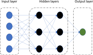
Empirical correlation for formation resistivity prediction using machine learning

Real-time static Poisson’s ratio prediction of vertical complex lithology from drilling parameters using artificial intelligence models

Estimating electrical resistivity from logging data for oil wells using machine learning
Explore related subjects.
- Artificial Intelligence
Data Availability
Most of the data are provided in the paper and a detailed sample will be provided upon request.
Abbreviations
Artificial intelligence
Average absolute percentage error
Adaptive neuro-fuzzy inference system
Artificial neural network
Sonic shear log (ms/ft)
Delta time compressional logs (ft, min)
Decision tree
Decision tree regression
Fuzzy logic
Gamma-ray (API)
Lateral log resistivity (Ω m)
Machine learning
Neutron porosity (pu)
Coefficient of correlation
Random forest
Bulk density (g/cm 3 )
Stock-tank oil initially in place
Lord, R.: Technological breakthroughs advanced upstream E&P’s evolution. J. Petrol. Technol. 59 (10), 111–116 (2007)
Article Google Scholar
Carpenter, C.: Production logging, openhole-log interpretation help discover new oil reserves. J. Petrol. Technol. 73 (08), 42–43 (2021)
Anderson, B.I., et al.: Dielectric inversion of LWD propagation-resistivity tools for formation evaluation. In: Paper presented at the SPWLA 63rd Annual Logging Symposium, Stavanger, Norway, June 2022. Paper Number: SPWLA-2022–0022. https://doi.org/10.30632/SPWLA-2022-0022 . 2022. OnePetro.
Zhao, P.; Qin, R.; Pan, H.; Ostadhassan, M.; Wu, Y.: Study on array laterolog response simulation and mud-filtrate invasion correction. Adv. Geo-Energy Res. 3 (2),175–186 (2019). https://doi.org/10.26804/ager.2019.02.07
Lander, L.; Silva, A.; Simon, C.: Resistivity logging in conductive-mud environment and high resistivity formations. Dual Laterolog or Propagation LWD Tool? Paper presented at the SPE Latin American and Caribbean Petroleum Engineering Conference, Quito, Ecuador, November 2015. Paper Number: SPE-177084-MS. https://doi.org/10.2118/177084-MS
Hu, G.; Bittar, M.; Hou, J.: Evaluation of horizontal wells using LWD propagation resistivity and laterolog-type resistivity logs. Paper presented at the SPE Annual Technical Conference and Exhibition, San Antonio, Texas, USA, September 2006. Paper Number: SPE-103150-MS. https://doi.org/10.2118/103150-MS
Zhen, Q.; Heping, P.; Aiping, W.; Huaijie, Y.; Ting, H.; Min, H.; Zhonghao, W.: Application of conventional propagation resistivity logging for formation boundary identification in geosteering. J. Geophys. Eng. 14 (5), 1233–1241 (2017). https://doi.org/10.1088/1742-2140/aa80a0
Sun, K.; Thiel, M.; Mirto, E.; Tan, S.; Liu, J.; Feng, Y.; Harms, K.; Nesttun, Ø.; Beate, P.; Tom, V.; Ashwin, T.; Farid, L.; Ruixia, W.; Hui, D.; Jean-Michel, W.; Vera, K.; Wang, H.; Wang, F.; Snovida, Z.; Beltran, G.; Eliana, C.; Pinzón, P.; Joaquín, A.; Delgado, H.J.; Liu, W.; Wang, J.; Dzevat, O.: New generation of ultra-high definition directional propagation resistivity for real time reservoir characterization and geosteering-while-drilling. Constr. Build. Mater. (2021). https://doi.org/10.2118/204739-MS
Moustafa, I.K.; Gutierrez, F.A.; Alfelasi, A.S.; Khemissa, H.; Mutwali, O.A.; Vargas, M.; Fares, W.; Clegg, N.; Ahmet, A.: Ultra-deep resistivity mapping tool provided geostopping solution to reduce uncertainty and eliminated the need for pilot holes for the first time offshore Abu Dhabi. In: Paper presented at the SPE/IADC Middle East Drilling Technology Conference and Exhibition, Abu Dhabi, UAE, May 2021. Paper Number: SPE-202133-MS (2021). https://doi.org/10.2118/202133-MS
Mohaghegh, S.: Virtual-intelligence applications in petroleum engineering: Part 1? Artificial neural networks. J. Petrol. Technol. 52 , 64–73 (2000). https://doi.org/10.2118/58046-MS
Khan, M.F.; Ashqar, A.A.; Rawahi, A.S.; Gashut, M.; Hammadi, K.E.: Advances in pulse neutron capture in evaluating formation properties within low permeability carbonates reservoir onshore Abu Dhabi: an integrated case study. Paper presented at the Abu Dhabi International Petroleum Exhibition & Conference, Abu Dhabi, UAE, November 2016. Paper Number: SPE-182985-MS. https://doi.org/10.2118/182985-MS
Anifowose, F.; Abdulazeez A.: Prediction of porosity and permeability of oil and gas reservoirs using hybrid computational intelligence models. In: Paper presented at the North Africa Technical Conference and Exhibition, Cairo, Egypt, February 2010 (2010). https://doi.org/10.2118/126649-MS
Ważny, J.; Stefaniuk, M.; Cygal, A.: Estimation of electrical resistivity using artificial neural networks: A case study from Lublin Basin. Se Poland. Acta Geophys. 69 (2), 631–642 (2021). https://doi.org/10.1007/s11600-021-00554-0
Ali, J.K.: Neural Networks: A New Tool for the Petroleum Industry? European Petroleum Computer Conference, Aberdeen, U.K., March (1994).
Anifowose, F. A.: Artificial intelligence application in reservoir characterization and modeling: whitening the black box. In: Paper presented at the SPE Saudi Arabia section Young Professionals Technical Symposium, Dhahran, Saudi Arabia, March 2011 (2011). https://doi.org/10.2118/155413-MS
Baneshi, M.; Behzadijo, M.; Schaffie, M.; Nezamabadi-Pour, H.: Predicting log data by using artificial neural networks to approximate petrophysical parameters of formation. Pet. Sci. Technol. 31 (12), 1238–1248 (2013). https://doi.org/10.1080/10916466.2010.540611
Anifowose, F.A.; Abdulraheem, A.; Al-Shuhail, A.; Denis P. S.: Improved permeability prediction from seismic and log data using artificial intelligence techniques. In: Paper presented at the SPE Middle East Oil and Gas Show and Conference, Manama, Bahrain, March 2013 (2013). https://doi.org/10.2118/164465-MS
Al-AbdulJabbar, A.; Elkatatny, S.; Mahmoud, M.; Abdulazeez A.: Predicting formation tops while drilling using artificial intelligence. In: Paper presented at the SPE Kingdom of Saudi Arabia Annual Technical Symposium and Exhibition, Dammam, Saudi Arabia, April 2018 (2018). https://doi.org/10.2118/192345-MS
Gowida, A.; Salaheldin, E.; Saad, A.-A.; Abdulazeez, A.: New computational artificial intelligence models for generating synthetic formation bulk density logs while drilling. Sustainability 12 (2), 686 (2020). https://doi.org/10.3390/su12020686
Download references
No External fund for this research and the authors would like to thank KFUPM for giving permission to publish this work.
Author information
Authors and affiliations.
Department of Petroleum Engineering, King Fahd University of Petroleum & Minerals, Dhahran, 31261, Saudi Arabia
Fawaz Alboghail, Abdulazeez Abdulraheem, Ahmed Farid Ibrahim, Salaheldin Elkatatny & Mohamed Mahmoud
Center for Integrative Petroleum Research, King Fahd University of Petroleum & Minerals, Dhahran, Saudi Arabia
Abdulazeez Abdulraheem, Ahmed Farid Ibrahim, Salaheldin Elkatatny & Mohamed Mahmoud
You can also search for this author in PubMed Google Scholar
Contributions
The manuscript was written through the contributions of all authors. All authors have approved the final version of the manuscript.
Corresponding author
Correspondence to Ahmed Farid Ibrahim .
Ethics declarations
Conflict of interest.
The authors declare that there is no conflict of interest regarding the publication of this paper.
Rights and permissions
Springer Nature or its licensor (e.g. a society or other partner) holds exclusive rights to this article under a publishing agreement with the author(s) or other rightsholder(s); author self-archiving of the accepted manuscript version of this article is solely governed by the terms of such publishing agreement and applicable law.
Reprints and permissions
About this article
Alboghail, F., Abdulraheem, A., Ibrahim, A.F. et al. Resistivity Log Prediction in Horizontal Low Formation Quality Well Using Data-Driven Robust Models. Arab J Sci Eng 48 , 9549–9557 (2023). https://doi.org/10.1007/s13369-023-07946-y
Download citation
Received : 23 July 2022
Accepted : 14 May 2023
Published : 10 June 2023
Issue Date : July 2023
DOI : https://doi.org/10.1007/s13369-023-07946-y
Share this article
Anyone you share the following link with will be able to read this content:
Sorry, a shareable link is not currently available for this article.
Provided by the Springer Nature SharedIt content-sharing initiative
- Machine learning algorithms
- Well logging
- Horizontal electrical resistivity
- Find a journal
- Publish with us
- Track your research
COMMENTS
There are a many approaches to construct the low frequency model to start the seismic inversion, such as: 1) using well-log only; 2) using well-log and seismic velocities; 3) using multi ...
Well logging has undergone constant and sweeping changes since its birth in 1927 in France (Tiab and Donaldson, 2004).Luthi (2001) summarizes the development history of well logging, and four distinct phases can be divided. (1) The conceptual phase (1921-1927) In order to understand the geological characteristics of the subsurface formation, there is in great need to record petrophysical ...
Origin and Production. James G. Speight Ph.D., D.Sc., in Natural Gas, 2007 2.2.4 Logging. Well logging is a method used for recording rock and fluid properties to find gas- and oil-containing zones in subterranean formations. Drilling of an exploratory or developing well is the first contact that a geologist has with the actual contents of the subsurface geology.
7.1 Well Logging. Well logging is an evaluation method in which a logging crew lowers a special tool, a sonde, into the well and then pulls it back up. As the sonde passes the formations on its way up the wellbore, it senses and measures electrical, radioactive, and acoustic (sound) properties of the rocks.
Explore the latest full-text research PDFs, articles, conference papers, preprints and more on WELL LOGGING. Find methods information, sources, references or conduct a literature review on WELL ...
Drilling deviated wells has become customary in recent times. This work condenses various highly deviated and horizontal well log interpretation techniques supported by field examples. Compared to that in vertical wells, log interpretation in highly deviated wells is complex because the readings are affected not only by the host bed but also the adjacent beds and additional wellbore-related ...
Abstract. Accelerators have been integral to subsurface probing for decades. Tools with deuterium-tritium (D-T) generators and scintillators utilizing gamma rays from thermal neutron capture, inelastic scattering, and activation are routine in cased-hole logging tools for reservoir and well monitoring to locate and quantify remaining hydrocarbons prior to initiating secondary or tertiary ...
With the advancements in well logging technologies, some innovative logging tools are now available to provide more data and information to geoscientists, drilling engineer and reservoir engineer for comprehensive assessment of shale reservoirs. ... (Timur-Coates or Coates) model, and (ii) the mean-T2 [the Schlumberger-Doll-Research (SDR ...
Well logging is a means of recording the physical, acoustic and electrical properties of the rocks penetrated by a well. It is carried out by service companies, which work under contract for the oil companies. Logging has the advantage that it measures in situ rock properties which cannot be measured in a laboratory from either core samples or cuttings.
Well logging. acoustic and electrical properties of the rocks. penetrated by a well. It is carried out by service. companies, which work under contract for the oil. companies. Logging has the ...
This Special Issue calls for theoretical and empirical papers focusing on the following topics: Results of well logging interpretation in various projects, interesting case studies; Well logging in the construction of digital models of rocks; Results of modeling to improve the inverse problem solution in well logging; Novelty in devices ...
This Special Issue on 'Rock Physics, Well Logging, and Formation Evaluation in Energy Exploration Systems' seeks high-quality works focusing on the latest novel advances for conventional and unconventional reservoir evaluation based on rock physics and well logging. Topics include, but are not limited to:
INTRODUCTION. Well logging is an integral part of formation evaluation inthat borehole measurements provide the largest source of data. These are usedwith core and fluid data to determine reservoir depth and thickness, porosity, lithology, hydrocarbon saturation, and permeability. This porosity, lithology, hydrocarbon saturation, and permeability.
The mismatching of well log and geochemical analysis results will give unreasonable prediction results providing the well log data are not calibrated with core analysis data (Gama and Schwark, 2023). The mismatching between core depth (drilling depth) and the well logging depth will result in significant errors ( Zhu et al., 2020 ; Gama and ...
In this Research Topic, it includes 10 articles addressing a variety of rock physics studies on unconventional resources, highlighting fundamental theories, laboratory work and well-log interpretation. The development of tight reservoirs is of significance to increase crude-oil production and optimize energy supply.
9781629810584. ISBN print: 089181664x. Publication date: January 01, 2002. This book provides examples of the use of well logs across a broad range of applications. The "Technology and Techniques" section includes papers on logging in high-angle wells and on logging and imaging while drilling. The "Sedimentology and Stratigraphy ...
tomography. The variation of a property down a borehole is recorded against depth as a log. Most logs are run by lowering the tool (measuring device) on a cable, often called wireline. In some situations, especially if the borehole is deviated far from the vertical, or may be unstable, the tool is placed in a modi ed.
This article is part of the Research Topic Advances in the Study of Natural Fractures in Deep and Unconventional Reservoirs View all 29 articles. Study on Well Logging Technology for the Comprehensive Evaluation of the "Seven Properties" of Shale Oil Reservoirs—An Example of Shale Oil in the Lucaogou Formation in the Jimsar Sag, Junggar ...
Keywords: well logging curves, LSTM, RNN, deep learning, digital well logging curve construction. Citation: Li J and Gao G (2023) Digital construction of geophysical well logging curves using the LSTM deep-learning network. Front. Earth Sci. 10:1041807. doi: 10.3389/feart.2022.1041807. Received: 11 September 2022; Accepted: 28 October 2022;
Well logging. Geophysical measurements in (deep) wells provide fundamental information for the interpretation of many geoscientific questions. Their interpretation enables the geophysical characterisation of the formations penetrated by the well, determining the position of sedimentary structures, as well as interpreting paleo-climatic conditions.
He is also a member of EAGE (European Association of Geoscientists &Engineers). His research interests include formation comprehensive evaluation, well logging data interpretation, ion conductivity and dielectric mechanism in rocks. He had authorized 4 patents and applied 12 patents in China, and 4 international patents.
Chapter 3G - Specialized Well-Logging Topics. Paul F. Worthington, Gaffney, Cline, and Assocs. Pgs. 379-420. ISBN 978-1-55563-120-8. Get permission for reuse. This chapter describes three categories of specialized well logging: downhole measurements that are concerned with the geometry and integrity of the wellbore; acoustic and electrical ...
My Library Topic Feeds Orders Account Settings Email Preferences Log Out Reading List Research shows that chronic workplace stress impacts our emotional well-being and can lead to physical health ...
Data for this work were obtained from LWD operations in the phase of drilling the 12″ section of a horizontal well. The predictive model was built on five inputs of logging parameters, namely: Gamma-ray "GR", Neutron porosity log "NPHI", Bulk-Density log "RHOB", Compressional wave transient slowness (i.e. the inverse of transient time) "DTC" and shear wave transient slowness ...