
The Greenhouse Effect Experiment
When it comes to our environment, it is so important that our children learn about the effects of climate change. One way we can start to educate them on environmental sciences is through a simple science experiment that creates the Greenhouse Effect in a jar. This activity is fantastic as a homeschool experiment, science fair project , classroom demonstration, and most importantly, as part of Earth Day lessons.
Climate Change Science Experiment
What you will discover in this article!

Disclaimer: This article may contain commission or affiliate links. As an Amazon Influencer I earn from qualifying purchases. Not seeing our videos? Turn off any adblockers to ensure our video feed can be seen. Or visit our YouTube channel to see if the video has been uploaded there. We are slowly uploading our archives. Thanks!
In recent years the climate crisis has become one of the most important challenges facing Earth and all of Earth’s inhabitants. Understanding how the greenhouse effect works is a fundamental lesson we need to be teaching all of our students. Throughout their lifetime they are going to witness massive environmental changes. Many of which, we have already seen in our lives. I can only imagine what is to come, and I know it weighs heavily on my tweens and teens. But through education and changing our practices and lifestyles, there are things we can all do to make a difference and protect our planet.
Let’s start with this science experiment that demonstrates the greenhouse effect.
Greenhouse Gas Science Experiment Video Tutorial
Check out our video of this climate change experiment exploring greenhouse gases and the greenhouse effect. If you can’t see the video, it is likely blocked by an adblocker. You can also view it on the STEAM Powered Family YouTube Channel .
What is the Greenhouse Effect?
First off, we need to explain the term: Greenhouse Effect . A greenhouse is a building with glass for the walls and roof. That glass structure traps heat inside, making it a great place to grow plants where it stays all warm and cozy, even after the sun goes down or it is cooler outside.
Instead of glass, our planet is surrounded by an atmosphere made up of gases. Like a great big puffy coat of gas wrapped around the entire planet. The atmosphere traps the sun’s heat on the Earth’s surface making our planet perfect for living organisms.
The balance of those gases is delicate, and due to a number of different factors, in particular the burning of fossil fuels, that balance is being disrupted and it is affecting the quality of that protective layer around our Earth.
One of the most important greenhouse gases is carbon dioxide. When we drive our cars and burn fossil fuels like gas and oil, we are putting more carbon dioxide into the atmosphere. This in turn causes more heat to be trapped on the Earth, leading to an increase in the average temperatures. This affects all living organisms, including humans.

The Greenhouse Effect Science Experiment
Now we know about the greenhouse effect, let’s do some science! For this experiment we are going to use our much beloved and simple, baking soda and vinegar chemical reaction .
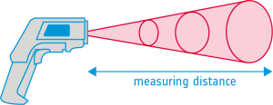
5 Large Jars – Using all 5 jars provides an opportunity to apply scientific theory and the scientific method . Vinegar – White, standard vinegar is best. Baking Soda – Also known as sodium bicarbonate or bicarb. Don’t use Baking Powder! It is a completely different chemical formula. You can learn more here about the differences between baking soda and baking powder . Measuring cups and spoons – Important for accuracy during testing. Plastic Wrap – Also known as clingfilm. It must be clear and able to seal tightly without tearing. I know we don’t want to use plastic, but in this case it is what we need for this science experiment. You can try it with other materials, but we struggled to get the desired results. You can always save the plastic and reuse it! Elastic bands – Large enough to fit over the mouth of the jar to secure the plastic wrap. Heat Source – You can use a sunny window sill if you live somewhere with lots of hot direct sunlight, or use a heat lamp, space heater, or in our case we used a heat vent/radiator. It just needs to provide lots of heat evenly between the jars. Thermometer – We have a non-contact infrared thermometer that worked perfectly. The kids LOVE using this type of thermometer in their science experiments but you can also use standard thermometers . If you use standard thermometers you will need one for each jar and a small knife or sharp scissors. Masking Tape and Sharpie – For labeling the jars
Prepare the Jars
Start by labeling the jars. You will want:
- Air (control)
- Vinegar (control)
- Baking Soda (control)
The fifth jar does not need to be labeled, that one you will also be doing the reaction in, but without the plastic covering. However, if you want to label it, go ahead!
The reason we are doing all of these controls, is that we want to show that it is not just the vinegar or just the baking soda, or just the chemical reaction causing our result. We want to prove it is the trapped carbon dioxide gas.
Prepare a piece of plastic wrap big enough to cover the mouth of the jar with a bit of extra down the sides so it can be sealed completely. Repeat for 4 jars. Also add an elastic band for each piece of plastic wrap.
Place plastic wrap on the air jar and secure it with an elastic.
Add 1/4 up of vinegar to the vinegar jar, then cover with plastic wrap and secure with an elastic.
Add 1 tablespoon of baking soda to the baking soda jar, cover with plastic wrap and secure with elastic.

Reaction Time!
This next step is easiest with two people. Have one person read with the plastic wrap and elastic. The other person will add the baking soda to the jar, then add the vinegar. VERY QUICKLY place the plastic wrap over the mouth of the jar and secure it with an elastic. We need to capture the gases from the reaction, so work fast!
Here comes the sun
Now place the jars in front of your heat source. Ensure they are positioned so they will all be heated evenly. We used a heat register/radiator to evenly apply heat. A windowsill in the bright sun would work well too. Leave the jars with the heat for 5 to 10 minutes. We tested at both the 5 minute and 10 minute mark.
This heat source is replicating the warming effect of the sun.
Chemical Reaction Comparison
While the four jars are warming, take your fifth jar. Add 1 tablespoon of baking soda and 1/4 cup of vinegar. Watch the bubbly reaction! After about 30 seconds take a temperature reading. What do you notice? Baking soda and vinegar is an endothermic reaction! This is extremely interesting in the context of this greater experiment.
Temperature check
After your jars are warmed, it is time to take temperature readings.
If you are using a non-contact infrared thermometer, have your students take temperature readings from each jar, we found it best to aim straight down into the jar.
If you are using a standard thermometer, make a small slit in the plastic top of each jar, just big enough to slip the thermometer in without letting too much air escape. Place a thermometer in each jar. Wait one minute, then remove the thermometer and check the temperature readings.
What do you notice about the temperature readings? Record your results!
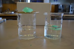
Greenhouse Effect Results
The chemical reaction in the enclosed jar is warmer than all the other jars with plastic covering. Those control jars are all about the same temperature. The coldest jar is the chemical reaction with no plastic covering. So cool!
The Greenhouse Science
The chemical reaction between baking soda and vinegar is an acid-base reaction. Baking soda is a base and vinegar is an acid. When we combine them, they react in a bubbly, endothermic reaction. Endothermic means it becomes colder during the reaction.
Here is the chemical formula of this reaction
C 2 H 4 O 2 + NaHCO 3 -> NaC 2 H 3 O 2 + H 2 O + CO 2 (g) vinegar + sodium bicarbonate -> sodium acetate + water + carbon dioxide(g)
The carbon dioxide is a gas, just like it is in the atmosphere, where it is one of the greenhouse gases.
In this experiment we are trapping the carbon dioxide gas in the jar. When heat is applied, the carbon dioxide traps more heat in the jar than our controls.
Where this became really interesting for us, was when the kids realized the reaction was endothermic, as demonstrated in our open chemical reaction jar. That means our jar with the trapped carbon dioxide not only trapped heat, but it trapped enough heat to counteract the endothermic reaction, and still make that jar warmer than the controls.
That is one powerhouse of a greenhouse effect!
Troubleshooting
If you have problems with this experiment there may be a few things to look at.
First, make sure your jars are being evenly heated. Depending on how you heat your jars, certain jars my be getting more heat than others. If you are using heat lamps, you may want to ensure you have one heat lamp per jar and place them equal distances from each jar.
If you used a standard thermometer, make sure your slit is not letting too much of the carbon dioxide out of the jar, it will take the heat with it.
When the reaction is triggered, make sure you act fast to get that plastic wrap on there and trap those gases!
Learning More About Climate Change
We really enjoy learning from NASA’s incredible resources. They have an entire site dedicated to climate and kids called Climate Kids that is packed with learning resources.
If you have Netflix, definitely look for any documentaries by David Attenborough . My tweens and teens have watched many of his documentaries and learned so much.
Tackle more Earth Day and Environmental Sciences projects with your kids, with our collection of Earth Day Activities .
Climate Change and Environmental Sciences Worksheets

Enjoy learning about our planet and start putting your lessons to work to protect our home. The more we know, the better we can all work to project our Earth.

More Educational Resources

5 Days of Smart STEM Ideas for Kids
Get started in STEM with easy, engaging activities.
Your browser is not supported
Sorry but it looks as if your browser is out of date. To get the best experience using our site we recommend that you upgrade or switch browsers.
Find a solution
- Skip to main content
- Skip to navigation
- Back to parent navigation item
- Primary teacher
- Secondary/FE teacher
- Early career or student teacher
- Higher education
- Curriculum support
- Literacy in science teaching
- Periodic table
- Interactive periodic table
- Climate change and sustainability
- Resources shop
- Collections
- Remote teaching support
- Starters for ten
- Screen experiments
- Assessment for learning
- Microscale chemistry
- Faces of chemistry
- Classic chemistry experiments
- Nuffield practical collection
- Anecdotes for chemistry teachers
- On this day in chemistry
- Global experiments
- PhET interactive simulations
- Chemistry vignettes
- Context and problem based learning
- Journal of the month
- Chemistry and art
- Art analysis
- Pigments and colours
- Ancient art: today's technology
- Psychology and art theory
- Art and archaeology
- Artists as chemists
- The physics of restoration and conservation
- Ancient Egyptian art
- Ancient Greek art
- Ancient Roman art
- Classic chemistry demonstrations
- In search of solutions
- In search of more solutions
- Creative problem-solving in chemistry
- Solar spark
- Chemistry for non-specialists
- Health and safety in higher education
- Analytical chemistry introductions
- Exhibition chemistry
- Introductory maths for higher education
- Commercial skills for chemists
- Kitchen chemistry
- Journals how to guides
- Chemistry in health
- Chemistry in sport
- Chemistry in your cupboard
- Chocolate chemistry
- Adnoddau addysgu cemeg Cymraeg
- The chemistry of fireworks
- Festive chemistry
- Education in Chemistry
- Teach Chemistry
- On-demand online
- Live online
- Selected PD articles
- PD for primary teachers
- PD for secondary teachers
- What we offer
- Chartered Science Teacher (CSciTeach)
- Teacher mentoring
- UK Chemistry Olympiad
- Who can enter?
- How does it work?
- Resources and past papers
- Top of the Bench
- Schools' Analyst
- Regional support
- Education coordinators
- RSC Yusuf Hamied Inspirational Science Programme
- RSC Education News
- Supporting teacher training
- Interest groups

- More navigation items
Modelling the greenhouse effect
In association with Nuffield Foundation
- No comments
Use this demonstration to illustrate the greenhouse effect and the role of carbon dioxide as a greenhouse gas
The demonstration includes two parts. In the first, students observe a model of the greenhouse effect in a greenhouse using transparent bottles containing air. In the second, they learn about the role of carbon dioxide by comparing the effects in two separate vessels containing air and carbon dioxide respectively.
The experiments in both parts demonstrate the greenhouse effect by comparing the temperature increases in suitable vessels containing the gases, on exposure to light from a powerful lamp.
Each part of the demonstration will take about 30 minutes. However, the second part can be started well before the first part has been completed if sufficient apparatus is available.
The experiments involve slow, gradual temperature increases. If the temperatures are monitored electronically, with data logging and a live display, the experiment can be allowed to proceed while the class carries on with other work. If ordinary thermometers or electronic thermometers with digital displays are used, the temperatures will have to be recorded at one minute intervals, requiring the attention of the class to time and record for the duration of the demonstrations.
For both parts
- Photoflood light bulb, 275 W, in a plain bulb holder (see notes 1 and 2 below)
- Temperature sensors with leads, 3, with data logger and computer display (see note 3)
- Plastic drink bottles, transparent, 1 dm 3 , x2 (see note 4)
- 2-hole bungs, to fit bottles (see note 4)
- Clock, with second hand
- Stand, boss and clamp, x2
- Beakers, 250 cm 3 , x2
- Black card discs, x2
Apparatus notes
- Photoflood bulbs are available from photographic suppliers on the internet, or from photography shops on the high street, at a cost of £10–15 each for a 275 W bulb. The bulb should be fitted in a plain bulb-holder suitably stabilised so that it stands securely on the demonstration bench, and is easily switched on and off by the demonstrator without disturbing the bulb.
- The photoflood bulb should be situated so that the three temperature sensors or thermometers can be placed equidistant from the bulb, as shown in figure 1 below.

Source: Royal Society of Chemistry
How to set up the apparatus to model the greenhouse effect in a greenhouse and compare temperature increases in each of the two bottles
- Check that all three temperature sensors show the same temperature on the computer display when placed in the same temperature environment. Fit two of the sensors through the rubber bungs that will fit into the drinks bottles. Each of the three temperature sensors should be wrapped with a lead (or prepared aluminium) foil ‘flag’. Each flag is made from a piece of lead foil about 3 x 2 cm such that after wrapping around the sensor, a flag approximately 1 cm wide and 2 cm high made of doubled foil is formed (see figure 2 below). The sensor should then be positioned so that the face of each flag will be perpendicular to the radiation from the bulb. The end result should be a set of three temperature sensors with flags that are as similar as possible. The sensors carrying their flags need to fit easily through the necks of the drinks bottles. The setting up of the datalogger and three temperature sensors will depend on the kit available in the school. The handbook for the datalogger will provide the necessary instructions. Suitable software should be used to display the temperature data as a function of time as three lines of different colour on screen(s) visible to the class. Two of the temperature sensors will be required again in part 2, but without the lead flags.
- The two drinks bottles for part 1 should be identical, colourless, transparent, PET plastic (recycling code 1) water bottles, fizzy drink bottles or similar, of 1 dm 3 capacity, capable of carrying a 2-hole rubber bung in the mouth (see figure 3). One hole is needed to carry the temperature sensor (or the thermometer if used), the other to allow air flow to prevent pressure build-up. One of the bottles should be painted matt black on one ‘side’ and allowed to dry thoroughly. The bottles should be secured in an upright position, without obscuring the light path from the lamp.

How to prepare the thermometers or temperature sensors and the half-painted bottle required for the first experiment
- Finally set up the apparatus for part 1 as in figure 1, clamping as necessary to ensure the arrangement is secure from accidental knocks, and at the appropriate point in the lesson, replace by the simple arrangement for part 2 as in figure 4. Note that the photoflood lamp is now positioned and clamped above the beakers, midway between them.

How to set up the apparatus to model the effect of carbon dioxide on temperature for the second experiment
- Lead foil pieces (TOXIC, DANGEROUS FOR THE ENVIRONMENT), about 3 cm x 2 cm, x3 (aluminium foil can be used as an alternative to lead foil but must be either painted black or darkened which happens after it has been in contact with food)
- Matt black paint (for example, blackboard paint)
- Source of carbon dioxide gas
- Methane (natural gas) (EXTREMELY FLAMMABLE)
- Pentane (EXTREMELY FLAMMABLE, HARMFUL, DANGEROUS FOR THE ENVIRONMENT), 1 cm 3
- Hexane (HIGHLY FLAMMABLE, HARMFUL, DANGEROUS FOR THE ENVIRONMENT), 1 cm 3
Health, safety and technical notes
- Read our standard health and safety guidance.
- Lead foil, Pb(s), (TOXIC, DANGEROUS FOR THE ENVIRONMENT) – see CLEAPSS Hazcard HC056 . In part 1 the lead foil pieces are for making the ‘flags’ around the temperature sensors (Note 3). The Lead foil can be replaced with darkened aluminium foil and the effect is still observed.
- Carbon dioxide, CO 2 (g) – see CLEAPSS Hazcard HC020a . For use of a carbon dioxide cylinder also see Laboratory Handbook Section 9.9 about the safe storage and use of gas cylinders. If using solid carbon dioxide (dry ice), this should be obtained within 24 hours of the demonstration in substantially larger quantity than required for the experiment, and stored in a vented insulated container until required. All handling must be done using thermal gloves and handling tongs. If neither a carbon dioxide cylinder nor a supply of dry ice is available, carbon dioxide gas may be generated chemically – see these standard techniques for generating, collecting and testing gases . Replace the thistle funnel shown with a tap funnel or an unstoppered separating funnel. Use about 10 g of small marble chips (calcium carbonate) and about 100 cm 3 of hydrochloric acid (2 M) for the carbon dioxide generator. Add the acid a few cm 3 at a time to the marble chips to generate a steady stream of carbon dioxide. Either shortly before part 2 of the demonstration, or as part of the demonstration, allow a flow of carbon dioxide to displace the air from the beaker. Alternatively pieces of solid carbon dioxide can be allowed to evaporate in the bottom of the beaker.
- Methane (Natural gas), CH 4 (g), (EXTREMELY FLAMMABLE) – see CLEAPSS Hazcard HC045a .
- Pentane, C 5 H 12 (l), (EXTREMELY FLAMMABLE, HARMFUL, DANGEROUS FOR THE ENVIRONMENT) – see CLEAPSS Hazcard HC045a.
- Hexane, C 6 H 14 (l), (EXTREMELY FLAMMABLE, HARMFUL, DANGEROUS FOR THE ENVIRONMENT) – see CLEAPSS Hazcard HC045a.
- With the apparatus set up as in figure 1 above, start the datalogging programme with all three sensors at the same time (which should all show the same temperature), and immediately switch on the photoflood lamp.
- Allow the datalogging to proceed with the graphical display visible to the class. Ensure the class are aware of which graphical trace belongs to which sensor. In about 15 minutes, the three traces should level off, the ‘bare’ sensor showing a typical increase of around 5°C, the clear bottle about 8°C, and the blackened bottle about 13°C.
- If two further temperature sensors and a second datalogger are available, part 2 can be demonstrated while part 1 is running. Alternatively the class can proceed with other tasks until there is a clear result from part 1 on the display screen.
- Reset the datalogger and software to start again with inputs from two temperature sensors.
- Start the datalogger and switch on the lamp; the two traces should remain together, though showing a gradual rise.
- When this gradual rise levels off, introduce carbon dioxide as a steady flow into one of the beakers. The trace from that beaker should soon show a higher temperature than the beaker with only air – typically up to 8 degrees higher. If the gas flow is stopped, the carbon dioxide will slowly diffuse out of the beaker, replaced by air, and the temperature should begin to fall again.
- (Optional) Clear the carbon dioxide from its beaker, and repeat 1 and 2 above. Ensure all sources of ignition have been removed. Now introduce a slow stream of methane from the gas tap into the beaker and observe the effect on the temperature trace.
- (Optional) Again repeat 1 and 2 above and ensure all sources of ignition have been removed. Use a dropping pipette to drop about 1 cm 3 of the volatile liquid into the beaker. This will slowly evaporate, and the effect on the temperature trace can be followed as it does so.
Teaching notes
In a garden greenhouse, visible light passes through the glass and is absorbed by darker surfaces inside. This absorbed energy heats up the materials, also warming the surrounding air. But convection is restricted by the enclosing glass and the inside temperature of the greenhouse rises. This is the main cause of warming in a garden greenhouse.
However, in addition the warm surfaces re-radiate some of the absorbed energy, but at longer wavelengths in the infrared region of the spectrum. Some of this infra-red radiation is absorbed by glass and contributes to the warming of the greenhouse. It is this latter effect that is called the ‘greenhouse effect’. The greenhouse effect in the Earth’s atmosphere is caused by a number of gases that behave in a similar way to glass. They are transparent to visible light, but absorb in part of the infrared spectrum. Some of these gases are listed in the table. It can be seen that carbon dioxide is the most important greenhouse gas because of its relatively high concentration in the atmosphere rather than its intrinsic greenhouse efficiency.
| Gas | Relative greenhouse efficiency per molecule | Concentration in the atmosphere/ppm | Relative efficiency x concentration/ppm |
|---|---|---|---|
| Carbon dioxide | 1 | 350 | 350 |
| Methane | 30 | 1.7 | 51 |
| Dinitrogen | 160 | 0.31 | 49.6 |
| Ozone | 2,000 | 0.06 | 120 |
| CFC 11 (CCI3F) | 21,000 | 0.00026 | 5.46 |
| CFC 12 (CCI2F2) | 25,000 | 0.00024 | 6 |
In part 1, the experiment demonstrates the situation in a greenhouse using a plastic bottle. It also shows the effect of a black surface absorbing the energy from visible light.
In part 2, however, replacing the plastic bottles with open beakers removes the restriction on convection. The difference in temperature rise between the two beakers comes mainly from absorption by the gases of the radiant (infra-red) energy from the lead discs at the bottom of the beakers
Water vapour, carbon dioxide and ozone are the most important of the greenhouse gases, the first two because of their relatively high concentration in the atmosphere rather than because of their intrinsic greenhouse efficiency – indeed water vapour accounts for more than a third of the overall greenhouse effect. However, methane also makes a significant contribution, and it is the increasing proportion of carbon dioxide, and to a lesser extent methane, that seems to be producing the effect of global warming.
Additional information
This is a resource from the Practical Chemistry project , developed by the Nuffield Foundation and the Royal Society of Chemistry.
Practical Chemistry activities accompany Practical Physics and Practical Biology .
© Nuffield Foundation and the Royal Society of Chemistry
- 11-14 years
- 14-16 years
- Demonstrations
- Environment
- Environmental science
Specification
- Greenhouse gases in the atmosphere maintain temperatures on Earth high enough to support life. Water vapour, carbon dioxide and methane are greenhouse gases.
- Describe the greenhouse effect in terms of the interaction of radiation with matter.
- 8.24 Describe how various gases in the atmosphere, including carbon dioxide, methane and water vapour, absorb heat radiated from the Earth, subsequently releasing energy which keeps the Earth warm: this is known as the greenhouse effect
- C1.3.1 describe the greenhouse effect in terms of the interaction of radiation with matter
- C6.2c describe the greenhouse effect in terms of the interaction of radiation with matter within the atmosphere
- C6.3c describe the greenhouse effect in terms of the interaction of radiation with matter within the atmosphere
- 2.3.6 recall that the percentage of carbon dioxide in the atmosphere has risen from 0.03% to 0.04% because of combustion of organic compounds and is believed to have caused global warming;
- 2.5.28 demonstrate knowledge that the combustion of fuels is a major source of atmospheric pollution due to: combustion of hydrocarbons producing carbon dioxide, which leads to the greenhouse effect causing sea level rises, flooding and climate change;…
- 2.5.26 demonstrate knowledge that the combustion of fuels is a major source of atmospheric pollution due to: combustion of hydrocarbons producing carbon dioxide, which leads to the greenhouse effect causing sea level rises, flooding and climate change…
- The greenhouse effect and the influence of human activity on it.
- Possible implications of increased greenhouse effect.
- 3. Illustrate how earth processes and human factors influence Earth’s climate, evaluate effects of climate change and initiatives that attempt to address those effects.
Related articles

How to teach atmospheric chemistry at 14–16
2024-02-06T06:00:00Z By Martin Bluemel
Use these guiding questions to guarantee student understanding of this tricky topic

Life cycle assessment of fast-food containers
2024-02-05T04:00:00Z By Nina Notman
Examining the environmental impact of single-use takeaway packaging

How science can make burial, cremation and memorial greener
2023-11-13T06:00:00Z By Kit Chapman
Does alkaline hydrolysis offer a more sustainable approach?
No comments yet
Only registered users can comment on this article., more experiments.

‘Gold’ coins on a microscale | 14–16 years
By Dorothy Warren and Sandrine Bouchelkia
Practical experiment where learners produce ‘gold’ coins by electroplating a copper coin with zinc, includes follow-up worksheet

Practical potions microscale | 11–14 years
By Kirsty Patterson
Observe chemical changes in this microscale experiment with a spooky twist.

Greenhouse effect experiment
In this activity pupils will undertake a controlled experiment to investigate how gases in the atmosphere affect the heat in an enclosed environment, by tracking the change in temperature of a glass jar containing carbon dioxide against a control jar. They will learn about the greenhouse effect and the role of carbon dioxide in Earth’s atmosphere.
This activity could be used as a main lesson activity, to introduce the concept of the Earth’s atmosphere, or as part of a series of lessons investigating environmental issues and the effect of global warming.
Show health and safety information
Please be aware that resources have been published on the website in the form that they were originally supplied. This means that procedures reflect general practice and standards applicable at the time resources were produced and cannot be assumed to be acceptable today. Website users are fully responsible for ensuring that any activity, including practical work, which they carry out is in accordance with current regulations related to health and safety and that an appropriate risk assessment has been carried out.
Show downloads
| Subject(s) | Climate Change, Design and technology, Science, Earth science |
|---|---|
| Age | 7-11 |
| Published | 2020 to date |
| Published by | |
| Collections | |
| Direct URL |
Share this resource
Did you like this resource.
Grade Level
Climate literacy principles, energy literacy principles, demos & experiments.


Have a question?
How do greenhouse gases trap heat in the atmosphere, greenhouse gas molecules in the atmosphere absorb light, preventing some of it from escaping the earth. this heats up the atmosphere and raises the planet’s average temperature..
February 19, 2021
What do CO 2 , methane, and water vapor have in common? If your first thought was “greenhouse gases,” you’d be correct! Greenhouse gases trap heat in the atmosphere, in a process called the “greenhouse effect.” 1 But how do these molecules actually warm our planet?
We’ll start our exploration of greenhouse gases with a single carbon dioxide (CO 2 ) molecule. Let’s say this CO 2 molecule came from the exhaust in your car. From your tailpipe, it drifts up into the atmosphere, diffusing among the other gases. There, particles of light—photons—hit our molecule.
So what happens to those photons? “Greenhouse gas molecules will absorb that light, causing the bonds between atoms to vibrate,” says Jesse Kroll, Professor of Civil and Environmental Engineering and Chemical Engineering at MIT. “This traps the energy, which would otherwise go back into space, and so has the effect of heating up the atmosphere.” Basically, the bonds between the carbon and oxygen atoms in our CO 2 molecule bend and stretch to absorb photons. (With other greenhouse gases, the molecular bonds are different, but in all cases, they absorb photons, stopping them from leaving the atmosphere.)
Eventually, our CO 2 molecule will release these photons. Sometimes, the photons continue out into space. But other times, they rebound back into the Earth’s atmosphere, where their heat remains trapped.
And importantly, greenhouse gases don’t absorb all photons that cross their paths. Instead, they mostly take in photons leaving the Earth for space. “CO 2 molecules absorb infrared light at a few wavelengths, but the most important absorption is light of about 15 microns,” says Kroll. Incoming light from the sun tends to have much shorter wavelengths than this, so CO 2 doesn’t stop this sunlight from warming the Earth in the first place. But when the Earth re-emits this light, 2 it has a longer wavelength, in the infrared spectrum.
And the range of wavelengths around 15 microns is a particularly crucial window. The most common greenhouse gas, water vapor, doesn’t efficiently absorb photons in this range. So when CO 2 grabs photons with wavelengths around 15 microns, it’s selecting for the same light that normally has the easiest time escaping Earth’s atmosphere.
There’s another reason why CO 2 is such an important greenhouse gas: it has a long atmospheric lifetime. This has to do with the way CO 2 reacts (or rather, doesn’t react) with the atmosphere. “The atmosphere is a very oxidative environment due to the presence of oxygen and ultraviolet radiation,” says Kroll. Oxidation occurs when oxygen steals electrons from another atom—it’s the same chemical reaction that causes iron to rust. Methane, another greenhouse gas, reacts easily with oxygen, which removes it from the atmosphere within around 12 years. That’s long enough to affect the climate, but nowhere near the lifetime of CO 2 , which does not react with oxygen and can last over a century.
CO 2 ’s long lifespan is the key reason that human activities are leading to climate change. As we keep taking carbon-based compounds like coal and oil out of the ground, and put that carbon in the atmosphere in the form of CO 2 , the added CO 2 piles up much faster than it can be naturally removed.
Thank you to Brittney Andrews of Clearlake, California, for the question. You can submit your own question to Ask MIT Climate here .
Read more Ask MIT Climate
1 This name is a little misleading. A real greenhouse traps heat because its glass stops the warm air inside from transferring heat to the colder surrounding air. Greenhouse gases don’t stop heat transfer in this way, but as this piece explains, in the end they have a similar effect on the Earth’s temperature.
2 Most of the sun’s radiation is absorbed by the Earth; only some is re-emitted as infrared light.

More Resources for Learning
Want to learn more.
Check out these related Explainers, written by scientists and experts from MIT and beyond.

Greenhouse Gases

Radiative Forcing

Related Pieces
How do clouds affect the earth's temperature are humans changing clouds, how do we know how much co2 was in the atmosphere hundreds of years ago, does the carbon dioxide that humans breathe out contribute to climate change, is today's climate change similar to the natural warming between ice ages, mit climate news in your inbox.

What Is the Greenhouse Effect?
Watch this video to learn about the greenhouse effect! Click here to download this video (1920x1080, 105 MB, video/mp4). Click here to download this video about the greenhouse effect in Spanish (1920x1080, 154 MB, video/mp4).
How does the greenhouse effect work?
As you might expect from the name, the greenhouse effect works … like a greenhouse! A greenhouse is a building with glass walls and a glass roof. Greenhouses are used to grow plants, such as tomatoes and tropical flowers.
A greenhouse stays warm inside, even during the winter. In the daytime, sunlight shines into the greenhouse and warms the plants and air inside. At nighttime, it's colder outside, but the greenhouse stays pretty warm inside. That's because the glass walls of the greenhouse trap the Sun's heat.

A greenhouse captures heat from the Sun during the day. Its glass walls trap the Sun's heat, which keeps plants inside the greenhouse warm — even on cold nights. Credit: NASA/JPL-Caltech
The greenhouse effect works much the same way on Earth. Gases in the atmosphere, such as carbon dioxide , trap heat similar to the glass roof of a greenhouse. These heat-trapping gases are called greenhouse gases .
During the day, the Sun shines through the atmosphere. Earth's surface warms up in the sunlight. At night, Earth's surface cools, releasing heat back into the air. But some of the heat is trapped by the greenhouse gases in the atmosphere. That's what keeps our Earth a warm and cozy 58 degrees Fahrenheit (14 degrees Celsius), on average.

Earth's atmosphere traps some of the Sun's heat, preventing it from escaping back into space at night. Credit: NASA/JPL-Caltech
How are humans impacting the greenhouse effect?
Human activities are changing Earth's natural greenhouse effect. Burning fossil fuels like coal and oil puts more carbon dioxide into our atmosphere.
NASA has observed increases in the amount of carbon dioxide and some other greenhouse gases in our atmosphere. Too much of these greenhouse gases can cause Earth's atmosphere to trap more and more heat. This causes Earth to warm up.
What reduces the greenhouse effect on Earth?
Just like a glass greenhouse, Earth's greenhouse is also full of plants! Plants can help to balance the greenhouse effect on Earth. All plants — from giant trees to tiny phytoplankton in the ocean — take in carbon dioxide and give off oxygen.
The ocean also absorbs a lot of excess carbon dioxide in the air. Unfortunately, the increased carbon dioxide in the ocean changes the water, making it more acidic. This is called ocean acidification .
More acidic water can be harmful to many ocean creatures, such as certain shellfish and coral. Warming oceans — from too many greenhouse gases in the atmosphere — can also be harmful to these organisms. Warmer waters are a main cause of coral bleaching .

This photograph shows a bleached brain coral. A main cause of coral bleaching is warming oceans. Ocean acidification also stresses coral reef communities. Credit: NOAA

Choose an Account to Log In

Notifications
Science project, greenhouse effect.

The Earth's climate has changed many times in the past. Subtropical forests have spread from the south into more temperate (or milder, cooler climates) areas. Millions of years later, ice sheets spread from the north covering much of the northern United States, Europe and Asia with great glaciers. Today, nearly all scientists believe human beings are changing the climate. How can that be? Over the past few centuries, people have been burning more amounts of fuels such as wood, coal, oil, natural gas and gasoline. The gases formed by the burning, such as carbon dioxide, are building up in the atmosphere. They act like greenhouse glass. The result, experts believe, is that the Earth heating up and undergoing global warming . How can you show the greenhouse effect?
What do you need?
- Two identical glass jars
- 4 cups cold water
- 10 ice cubes
- One clear plastic bag
- Thermometer
What to do?
- Take two identical glass jars each containing 2 cups of cold water.
- Add 5 ice cubes to each jar.
- Wrap one in a plastic bag (this is the greenhouse glass).
- Leave both jars in the sun for one hour.
- Measure the temperature of the water in each jar.
What you'll discover!
In bright sunshine, the air inside a greenhouse becomes warm. The greenhouse glass lets in the sun's light energy and some of its heat energy. This heat builds up inside the greenhouse. You just showed a small greenhouse effect . What could happen if this greenhouse effect changed the Earth's climate? Another version of a greenhouse is what happens inside an automobile parked in the sun. The sun's light and heat gets into the vehicle and is trapped inside, like the plastic bag around the jar. The temperature inside a car can get over 120 degrees Fahrenheit (49 degrees Celsius).
For more about Global Climate Change, visit the State of California's Climate Change Portal at: http://www.climatechange.ca.gov .
Related learning resources
Add to collection, create new collection, new collection, new collection>, sign up to start collecting.
Bookmark this to easily find it later. Then send your curated collection to your children, or put together your own custom lesson plan.
The greenhouse effect and its consequences – Investigating global warming

In this set of three activities, students will do hands-on experiments and learn how to interpret satellite images for better understanding the overall effects of global warming. In activity 1 students will make a model to demonstrate the greenhouse effect by showing that a higher level of carbon dioxide (CO2) means a higher temperature. The experiment will be complemented by the interpretation of satellite images showing the Earth’s CO2 levels at different time periods. Students will then learn about some of the consequences of an increased greenhouse effect – ice melting and changing albedo values. Students will explore these topics in activities 2 and 3.
Subject Geography, Physics, Science
- What the greenhouse effect is and how human activity changes the energy balance in Earth’s atmosphere
- The potential effects of increased levels of carbon dioxide on the Earth’s climate
- Possible consequences of the increased greenhouse effect
- The different consequences of flooding and rising sea water level due to melting sea-ice and melting ice sheets and glaciers
- What albedo is and how the reflectivity of different surfaces affect temperature
- How Earth observation can be used to monitor Earth’s climate
- 2 1L flasks
- Corks with hole for holding the thermometer
- 1 lamp with a heating bulb (more than 100W)
- 2 thermometers (0.10C precision)
- Acetic acid 32%
- Baking powder
- Ice cubes (optional)
- 4 glass beakers 250 ml
- Metal net with a diameter slightly bigger than the beakers
- Coloured ice cubes
- Table salt (NaCl)
- Tea-spoon or spatula to stir with
- IR-thermometer
- Pieces of paper or cardboard with different grey tones and different colours (see annex II)
- Lamp with heat bulb (if not sunny)
Did you know?
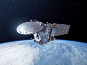
EarthCARE is an ESA mission that will improve our understanding of the role that clouds and aerosols play in both reflecting solar radiation back into space and trapping infrared radiation emitted from Earth’s surface. EarthCARE – the Earth Cloud Aerosol and Radiation Explorer – is being developed in collaboration with ESA and the Japan Aerospace Exploration Agency, JAXA. EarthCARE will collect global observations of cloud and aerosol profiles together with solar and thermal radiation to include these parameters in numerical weather and climate models. In addition, EarthCARE aerosol data will be valuable for monitoring air-quality.
One year on Earth – Understanding seasons
Brief description This resource includes two activities to foster and enhance pupils’ knowledge of seasons, and focuses on the basic...

Helping to manage water
Discover how satellites can help collecting information on water resources at over large areas.

Ocean views
Ice and snow can be a hot topic when talking about climate. The polar regions are very fragile and can tell us a lot about how Earth’s climate is changing. Andrew Shepherd of the University...

Paxi – The Greenhouse effect
Brief description:Join Paxi as he explores the greenhouse effect to learn about global warming. In this video, targeted at children...

The Power of Earth Observation
We are all intricately interconnected to our Earth – from the trees that provide us with oxygen, to the natural sources that shape our landscape. ESA’s Earth observation programme is at the forefront of monitoring...

A Passage opens – Arctic sea ice and climate change
Brief description In this set of three activities, students will discover the important role Arctic sea ice plays in the...
- Privacy Overview
- Strictly Necessary Cookies
This website uses cookies so that we can provide you with the best user experience possible. Cookie information is stored in your browser and performs functions such as recognising you when you return to our website and helping our team to understand which sections of the website you find most interesting and useful.
Strictly Necessary Cookie should be enabled at all times so that we can save your preferences for cookie settings.
If you disable this cookie, we will not be able to save your preferences. This means that every time you visit this website you will need to enable or disable cookies again.
The Greenhouse Effect and our Planet
The greenhouse effect happens when certain gases, which are known as greenhouse gases, accumulate in Earth’s atmosphere. Greenhouse gases include carbon dioxide (CO 2 ), methane (CH 4 ), nitrous oxide (N 2 O), ozone (O 3 ), and fluorinated gases.
Biology, Ecology, Earth Science, Geography, Human Geography
Loading ...

Earth keeps getting warmer. Scientists believe this is caused by an increase in something called greenhouse gases .
Greenhouse gases collect in Earth's atmosphere . The atmosphere is a layer of gases that surround Earth. Carbon dioxide (CO 2 ), methane (CH 4 ), and ozone (O 3 ), are kinds of greenhouse gases.
The greenhouse gases allow the sun's light to shine onto Earth's surface. Some of that heat gets reflected . It bounces from the surface of Earth. Then, the gases trap the heat inside Earth. The gases act like the glass walls of a greenhouse. In other words, they are warming.
Animals and Plants Contribute to Greenhouse Gases Without the greenhouse effect , Earth's average temperature would drop. Now, it is about 57 degrees Fahrenheit (14 degrees Celsius). It could drop to as low as 0 degrees Fahrenheit (minus 18 degrees Celsius). The weather would go from mild to very cold.
Some greenhouse gases come from nature. Animals and plants release carbon dioxide when they breathe. Methane is another greenhouse gas . It is released when soil and living things break down. Volcanoes also release greenhouse gases .
Factories and Vehicles Can also Be Blamed The Industrial Revolution happened in the late 1700s and early 1800s. This led to more factories and machines being built. The factories burned fuel and released more greenhouse gases into the atmosphere.
Greenhouse gases almost doubled between 1970 and 2004.
The amount of CO 2 in the atmosphere is growing. There is more CO 2 now than Earth has seen over the last 650,000 years.
Much of the CO 2 comes from burning fossil fuels . Cars, trains and planes all burn fossil fuels, such as gasoline. Many electric power plants do as well.
More Gases Lead to Global Warming Humans also release CO 2 into the atmosphere when they cut down forests . Trees contain large amounts of carbon.
People add methane to the atmosphere through farming of livestock such as cows. It also happens when we mine for coal .
Fluorinated gases are also greenhouse gases . Chlorofluoro carbons (CFCs) are one example of these. CFCs are used in refrigerators, air conditioners and aerosol cans .
As greenhouse gases increase, so does Earth's temperature. This rise caused by humans is known as global warming.
The Greenhouse Effect and Climate Change Even small increases in temperatures can have huge effects.
Perhaps the biggest effect is that glaciers and ice caps melt faster than usual. The meltwater d rains into the oceans . This causes sea levels to rise.
Glaciers and ice caps cover about one-tenth of the world's land. If all this ice melted, sea levels would rise about 70 meters (230 feet).
Climate scientists say that the world's sea level has risen.
Rising sea levels cause flooding in coastal cities. This could force millions of people in lower-lying areas out of their homes.
Millions of more people in countries depend on water from melted glaciers . They use it for drinking and watering crops . Losing these glaciers would greatly hurt those countries.
Greenhouse gases also cause changes in rain and snow .
In the 1900s, rain and snow increased in eastern parts of North and South America. It also increased in Northern Europe, and northern and Central Asia. However, it decreased in parts of Africa and southern Asia.
As climates change, so do environments . Animals that are used to a certain climate could become threatened.
Many humans depend on predictable rain patterns. This helps them to grow specific crops. If the climate of an area changes, the people there may no longer be able to grow anything. Some of them depend on farming for survival.
What Can We Do?
- Drive less. Use public transportation , carpool, walk, or ride a bike.
- Fly less. Airplanes produce huge amounts of greenhouse gas emissions.
- Reduce, reuse, and recycle .
- Plant a tree. Trees absorb carbon dioxide, keeping it out of the atmosphere.
- Use less electricity .
- Eat less meat. Cows are one of the biggest methane producers.
- Support alternative energy sources that don’t burn fossil fuels.
Artificial Gas
Chlorofluorocarbons (CFCs) are the only greenhouse gases not created by nature. They are created through refrigeration and aerosol cans.
CFCs, used mostly as refrigerants, are chemicals that were developed in the late 19th century and came into wide use in the mid-20th century.
Other greenhouse gases, such as carbon dioxide, are emitted by human activity, at an unnatural and unsustainable level, but the molecules do occur naturally in Earth's atmosphere.
Media Credits
The audio, illustrations, photos, and videos are credited beneath the media asset, except for promotional images, which generally link to another page that contains the media credit. The Rights Holder for media is the person or group credited.
Illustrators
Educator reviewer, last updated.
August 21, 2024
User Permissions
For information on user permissions, please read our Terms of Service. If you have questions about how to cite anything on our website in your project or classroom presentation, please contact your teacher. They will best know the preferred format. When you reach out to them, you will need the page title, URL, and the date you accessed the resource.
If a media asset is downloadable, a download button appears in the corner of the media viewer. If no button appears, you cannot download or save the media.
Text on this page is printable and can be used according to our Terms of Service .
Interactives
Any interactives on this page can only be played while you are visiting our website. You cannot download interactives.
Related Resources
Remember Me
Shop Experiment Exploring the Greenhouse Effect Experiments
Exploring the greenhouse effect.
Experiment #4 from Climate and Meteorology Experiments

Introduction
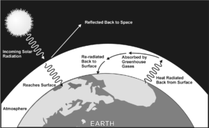
The greenhouse effect is a natural phenomenon that occurs due to solar radiation entering our atmosphere and interacting with specific atmospheric gases. When solar radiation reaches the upper layers of the atmosphere, short wavelength radiation passes through to the surface, while longer wavelength radiation is reflected back into space.
At night, the air above the surface cools and energy is transferred from the land to the air. Gases in the atmosphere keep the heat from radiating back into space, causing the air to be warmer than it otherwise would be if there were no atmosphere as shown in Figure 1. The gases most responsible for this effect are water vapor, carbon dioxide, methane, and nitrous oxide, also known as greenhouse gases.
- Use temperature sensors to measure temperatures in a model greenhouse and a control.
- Use the results to make conclusions about the greenhouse effect.
Sensors and Equipment
This experiment features the following sensors and equipment. Additional equipment may be required.

Correlations
Teaching to an educational standard? This experiment supports the standards below.
Ready to Experiment?
Ask an expert.
Get answers to your questions about how to teach this experiment with our support team.
- Call toll-free: 888-837-6437
- Chat with Us
- Email [email protected]
Purchase the Lab Book
This experiment is #4 of Climate and Meteorology Experiments . The experiment in the book includes student instructions as well as instructor information for set up, helpful hints, and sample graphs and data.
The Greenhouse Effect and our Planet
The greenhouse effect happens when certain gases, which are known as greenhouse gases, accumulate in Earth’s atmosphere. Greenhouse gases include carbon dioxide (CO 2 ), methane (CH 4 ), nitrous oxide (N 2 O), ozone (O 3 ), and fluorinated gases.
Biology, Ecology, Earth Science, Geography, Human Geography
Loading ...
The greenhouse effect happens when certain gases , which are known as greenhouse gases , accumulate in Earth’s atmosphere . Greenhouse gases include carbon dioxide (CO 2 ), methane (CH 4 ), nitrous oxide (N 2 O), ozone (O 3 ), and fluorinated gases.
Greenhouse gases allow the sun’s light to shine onto Earth’s surface, and then the gases, such as ozone, trap the heat that reflects back from the surface inside Earth’s atmosphere. The gases act like the glass walls of a greenhouse—thus the name, greenhouse gas
According to scientists, the average temperature of Earth would drop from 14˚C (57˚F) to as low as –18˚C (–0.4˚F), without the greenhouse effect.
Some greenhouse gases come from natural sources, for example, evaporation adds water vapor to the atmosphere. Animals and plants release carbon dioxide when they respire, or breathe. Methane is released naturally from decomposition. There is evidence that suggests methane is released in low-oxygen environments , such as swamps or landfills . Volcanoes —both on land and under the ocean —release greenhouse gases, so periods of high volcanic activity tend to be warmer.
Since the Industrial Revolution of the late 1700s and early 1800s, people have been releasing larger quantities of greenhouse gases into the atmosphere. That amount has skyrocketed in the past century. Greenhouse gas emissions increased 70 percent between 1970 and 2004. Emissions of CO 2 , rose by about 80 percent during that time.
The amount of CO 2 in the atmosphere far exceeds the naturally occurring range seen during the last 650,000 years.
Most of the CO 2 that people put into the atmosphere comes from burning fossil fuels . Cars, trucks, t rains , and planes all burn fossil fuels. Many electric power plants do as well. Another way humans release CO 2 into the atmosphere is by cutting down forests , because trees contain large amounts of carbon.
People add methane to the atmosphere through livestock farming, landfills, and fossil fuel production such as coal mining and natural gas processing. Nitrous oxide comes from agriculture and fossil fuel burning. Fluorinated gases include chlorofluorocarbons (CFCs), hydrochlorofluorocarbons (HCFCs), and hydrofluorocarbons (HFCs). They are produced during the manufacturing of refrigeration and cooling products and through aerosols.
All of these human activities add greenhouse gases to the atmosphere. As the level of these gases rises, so does the temperature of Earth. The rise in Earth’s average temperature contributed to by human activity is known as global warming .
The Greenhouse Effect and Climate Change Even slight increases in average global temperatures can have huge effects.
Perhaps the biggest, most obvious effect is that glaciers and ice caps melt faster than usual. The meltwater drains into the oceans, causing sea levels to rise.
Glaciers and ice caps cover about 10 percent of the world’s landmasses. They hold between 70 and 75 percent of the world’s freshwater . If all of this ice melted, sea levels would rise by about 70 meters (230 feet).
The Intergovernmental Panel on Climate Change states that the global sea level rose about 1.8 millimeters (0.07 inches) per year from 1961 to 1993, and about 3.1 millimeters (0.12 inches) per year since 1993.
Rising sea levels cause flooding in coastal cities, which could displace millions of people in low-lying areas such as Bangladesh, the U.S. state of Florida, and the Netherlands.
Millions more people in countries like Bolivia, Peru, and India depend on glacial meltwater for drinking, irrigation , and hydroelectric power . Rapid loss of these glaciers would devastate those countries.
Greenhouse gas emissions affect more than just temperature. Another effect involves changes in precipitation , such as rain and snow .
Over the course of the 20th century, precipitation increased in eastern parts of North and South America, northern Europe, and northern and central Asia. However, it has decreased in parts of Africa, the Mediterranean, and southern Asia.
As climates change, so do the habitats for living things. Animals that are adapted to a certain climate may become threatened. Many human societies depend on predictable rain patterns in order to grow specific crops for food, clothing, and trade. If the climate of an area changes, the people who live there may no longer be able to grow the crops they depend on for survival. Some scientists also worry that tropical diseases will expand their ranges into what are now more temperate regions if the temperatures of those areas increase.
Most climate scientists agree that we must reduce the amount of greenhouse gases released into the atmosphere. Ways to do this, include:
- driving less, using public transportation , carpooling, walking, or riding a bike.
- flying less—airplanes produce huge amounts of greenhouse gas emissions.
- reducing, reusing, and recycling.
- planting a tree—trees absorb carbon dioxide, keeping it out of the atmosphere.
- using less electricity .
- eating less meat—cows are one of the biggest methane producers.
- supporting alternative energy sources that don’t burn fossil fuels.
Artificial Gas
Chlorofluorocarbons (CFCs) are the only greenhouse gases not created by nature. They are created through refrigeration and aerosol cans.
CFCs, used mostly as refrigerants, are chemicals that were developed in the late 19th century and came into wide use in the mid-20th century.
Other greenhouse gases, such as carbon dioxide, are emitted by human activity, at an unnatural and unsustainable level, but the molecules do occur naturally in Earth's atmosphere.
Media Credits
The audio, illustrations, photos, and videos are credited beneath the media asset, except for promotional images, which generally link to another page that contains the media credit. The Rights Holder for media is the person or group credited.
Illustrators
Educator reviewer, last updated.
August 21, 2024
User Permissions
For information on user permissions, please read our Terms of Service. If you have questions about how to cite anything on our website in your project or classroom presentation, please contact your teacher. They will best know the preferred format. When you reach out to them, you will need the page title, URL, and the date you accessed the resource.
If a media asset is downloadable, a download button appears in the corner of the media viewer. If no button appears, you cannot download or save the media.
Text on this page is printable and can be used according to our Terms of Service .
Interactives
Any interactives on this page can only be played while you are visiting our website. You cannot download interactives.
Related Resources
November 9, 2023
23 min read
The Woman Who Demonstrated the Greenhouse Effect
Eunice Newton Foote showed that carbon dioxide traps the heat of the sun in 1856, beating the so-called father of the greenhouse effect by at least three years. Why was she forgotten?
By Zoe Kurland , Katie Hafner , Elah Feder & The Lost Women of Science Initiative

Paula Mangin
In 1856, decades before the term “greenhouse gas” was coined, Eunice Newton Foote demonstrated the greenhouse effect in her home laboratory. She placed a glass cylinder full of carbon dioxide in sunlight and found that it heated up much more than a cylinder of ordinary air. Her conclusion: more carbon dioxide in the atmosphere results in a warmer planet.
Several years later a Irish scientist named John Tyndall conducted a far more complicated experiment that demonstrated the same effect and revealed how it worked. Today Tyndall is widely known as the man who discovered the greenhouse gas effect. There’s even a crater on the moon named for him! Newton Foote, meanwhile, was lost to history—until an amateur historian stumbled on her story.
LISTEN TO THE PODCAST
On supporting science journalism
If you're enjoying this article, consider supporting our award-winning journalism by subscribing . By purchasing a subscription you are helping to ensure the future of impactful stories about the discoveries and ideas shaping our world today.
[ New to this season of Lost Women of Science? Listen to the most recent episodes on Flemmie Kittrell and Rebecca Lee Crumpler . ]
Lost Women of Science is produced for the ear. Where possible, we recommend listening to the audio for the most accurate representation of what was said.
EPISODE TRANSCRIPT
Zoe Kurland: About 12 years ago, Ray Sorenson was flipping through The Annual of Scientific Discovery of 1857. This is the kind of stuff Ray reads for fun, 19th Century science books and journals.
Ray Sorenson: You know, you buy a couple of those things, and you get hooked. I probably have a thousand publications that predate the Civil War.
Zoe Kurland: The Annual of Scientific Discovery was kind of a yearbook of all the science happenings from the previous year. And as Ray was perusing this stimulating tome, as one does, one particular entry caught his attention. It was about experiments conducted by someone named Eunice Foote.
Ray Sorenson: Let’s see where do I have it?
Zoe Kurland : He’s going to read us a few lines once he finds it.
Ray Sorenson: Ah, here it is. I think. I need my reading glasses. Hold on.
Zoe Kurland: So for context, what you’re about to hear is a write-up of a presentation of Eunice’s work that was given at a meeting in 1856. And Eunice didn’t get to read the paper herself at that meeting. A man actually read it for her. It was 1856, so you know.
Ray Sorenson: And I quote the whole thing: Professor Henry then read a paper by Mrs. Eunice Foote, prefacing it with a few words to the effect that science was of no country and of no sex. The sphere of woman embraces not only the beautiful and the useful, but the true. Mrs. Foote had determined first that the action… [fades]
Zoe Kurland: The paper goes on to describe an experiment by this Eunice Foote, which she conducted in her home laboratory, showing that water vapor and carbon dioxide trapped more heat than other gasses. And her conclusion-
Ray Sorenson: An atmosphere of that gas would give to our earth a much higher temperature and if there once was… [fades]
Zoe Kurland: Ray realized this unknown woman, Eunice Foote, had demonstrated the greenhouse gas effect in 1856. Which was odd because as far as most people knew, the person who first demonstrated it was someone named John Tyndall. He’s been called the father of the greenhouse effect or even the father of climate science. But John Tyndall started his experiments in 1859, and what Ray was looking at suggested Eunice had demonstrated the effect at least three years before that.
So who was this woman? And why had Ray heard of John Tyndall but not of her?
Ray Sorenson: There's no record of her. So I started digging around trying to find out stuff. And then I started thinking, okay, well she's, you know, if she's the first one to do this, she needs to be given credit for it.
Zoe Kurland: Ray wrote up a short paper on his discovery, hoping it might inspire at least one researcher to dig into the history of Eunice Foote. It went far beyond that. He got one, then another, and another.
Ray Sorenson: It's almost becoming competitive! [Laughs]
Zoe Kurland: And today, we throw our hat in the ring with the story of Eunice: how the mother of the greenhouse gas effect got lost and found.
Katie Hafner: This is Lost Women of Science. I’m Katie Hafner, and today, I’m joined by Zoe Kurland, who brings us the story of Eunice Newton Foote.
Zoe Kurland: In 1856, Scientific American described the work of a female scientist. They start with the obligatory – you know how people think women can’t do science? Well, guess what! Given the opportunity, some totally can! Not in those exact words, but that’s the gist. And their example? Mrs. Eunice Foote.” The article goes on to describe Eunice’s recent experiments with gasses.
They write, quote, “The columns of the Scientific American have been oftentimes graced with articles on scientific subjects, by ladies, which would do honor to men of the highest scientific reputation; and the experiments of Mrs. Foot [sic] afford abundant evidence of the ability of woman to investigate any subject with originality and precision.”
Pretty glowing review of Eunice’s work.
Katie Hafner: And it just happens to be Scientific American, our esteemed publishing partner. Hey Jeff.
Zoe Kurland: Hello Jeff. So how did Eunice Newton Foote make this discovery, land in the pages of the very prestigious Scientific American, and then get almost instantly overwritten by John Tyndall?
Katie Hafner: Yeah, I was going to ask that. How did that happen? I’ve never heard of that happening where men kind of take stuff over, but yeah, let’s hear the story.
Zoe Kurland: Alright, let’s take a step back.
Eunice Newton was born in Goshen, Connecticut in 1819. Eunice’s father was a cattle runner, and Connecticut wasn’t exactly booming, so when Eunice was three years old, her father, Isaac -- yes, his name was Isaac Newton -- her mother Thirza, and her ten brothers and sisters, hit the road in a covered wagon and headed to Bloomfield, New York. Which turned out to be a lucky move for Eunice.
Sally Kohlstedt: New York between 1830 and 1860. I mean, it was the progressive dynamo of- of much of the United States.
Zoe Kurland: Sally Kohlstedt is a science historian and a professor emeritus at the University of Minnesota.
Sally Kohlstedt: That's where the Underground Railroad went through to Canada. You know, that's where all these utopian religions were founded and things like the Oneida community with mixed marriages. So whether it was sex or religion or science or civil rights, it was all, all being discussed there. It would've been fun to live there.
Zoe Kurland: And Eunice’s family invested in her education. They even sent her to the first school in the country founded to provide young women with an education comparable to that of college-educated young men: The Troy Female Seminary.
And not only that, the Troy Female Seminary was right next to Rensselaer Polytechnic – the premiere science institute in the country at the time. And Troy students could go over there and take classes sometimes.
We’ve seen different accounts of exactly what age she was when she attended, but this would have been around the 1830s. A pretty big opportunity for a woman to get at the time.
Sally Kohlstedt: So she would have had a very unusual set of access points to sort of learn about and know what was going on.
Zoe Kurland: But even with this education, there was a feeling among the students at the Troy Seminary, documented in their letters, that all of this science education was great, but it was also sort of a tease.
John Perlin: And the biggest complaint was what the hell, we’re learning all the scientific stuff and then when we graduate, all available to us will be, you know, looking pretty.
Zoe Kurland: John Perlin teaches physics at UC Santa Barbara. He’s writing a book about Eunice.
John Perlin: You know, what outlet would we have because of the times.
Zoe Kurland: Even though the Troy School was different, these learned women still found themselves graduating into a world where they would be expected to cook and clean and needlepoint and smell nice and whatever. The “woman’s sphere” was still very much the “private sphere” -- the home. But Eunice managed to escape that life. In part, because of the man she married.
It all goes back to her father, Isaac Newton, the homesteader, and his perennial financial problems. Upstate New York hadn’t worked out much better than Connecticut for Isaac. He’d made some bad financial decisions, and then he passed away in 1835, leaving his family with a pile of debt. Soon, the Newton farm was about to go into foreclosure.
But Amanda, Eunice’s older sister, was like, I’m going to fix this and hired an attorney. One Elisha Foote. And yes, that is a man’s name. Our senior producer, Elah, tells us it was actually the name of her uncle.
John Perlin: He was ten years older than Eunice, and he was the district attorney of Seneca Falls. And he was moonlighting in Canandaigua where there was a federal court. And he took on their case, won it, and also won the hand of Eunice.
Zoe Kurland: In 1841, Eunice and Elisha got married. She was twenty-two years old and he was thirty-two. And they moved to Seneca Falls, New York, where Eunice soon found herself in the epicenter of the American women’s rights movement. One of their neighbors was Elizabeth Cady Stanton herself. Eunice got to know her just as Elizabeth’s star was beginning to rise.
They actually had a few connections. Elisha had studied law under Daniel Cady, Elizabeth’s father, and Eunice and Elizabeth had both attended the progressive Troy Female Seminary. We don’t know exactly how close they were, but living in Seneca Falls, they definitely knew each other.
Sally Kohlstedt: It's a very tiny town. You're really struck by how small the town is but therefore, how intimate it would've been for women to know each other.
Zoe Kurland: So in 1848, when Elizabeth Cady Stanton co-organized the country’s first ever women’s rights convention right there in Seneca Falls, Eunice was there. Elisha too.
Three-hundred people in all attended, mostly locals. At the convention, Elizabeth Cady Stanton and Lucretia Mott presented the Declaration of Sentiments, a list of demands and resolutions to be put forward for signatures, demands like the right to vote. It was modeled after the Declaration of Independence. But in the opening, it says “We hold these truths to be self-evident: that all men and women are created equal” and that basically, women were fed up with the tyranny of men.
Eunice’s name appears in the ladies section, right under Elizabeth Cady Stanton’s, and Elisha’s in the gentlemen’s, right above Frederick Douglass.
Katie Hafner: What do you know, Frederick Douglass makes a cameo appearance in this episode. He’s also all over another episode on Dr. Sarah Loguen Fraser.
Zoe Kurland: Well, you know, cool people always know what parties to show up to, so I’m not surprised.
Katie Hafner: That’s true.
Zoe Kurland: So Eunice is in a really good place for a woman to be at this point in time.
Sally Kohlstedt: She was immersed in a world that accepted her that gave herself confidence, I think, and that took her seriously. I think that's the important point that I see as I look back at her life. I thought some part of it is you have to be really pretty brilliant and pretty smart and pretty persistent to do that kind of work. On the other hand, if you're not at all supported, it can be extremely tough. And she doesn't seem to have had that problem.
Zoe Kurland: Okay, she’s an early feminist with a feminist husband. She has a great education. And then, she runs a little experiment in her home lab -- with huge ramifications.
That’s after the break.
Zoe Kurland: Elisha and Eunice were a bit of a power couple in Seneca Falls. They had a family together. They did feminism together. And they were both inventors and often collaborators. Among their inventions over the years were: a rubber shoe insert, a paper-making machine, an innovative ice skate.
Katie Hafner: This is incredible. I love people who invent things.
Zoe Kurland: I mean, not to romanticize them too much, ‘cause this is like the 1800s, I don’t want to be back there. But, this is hot. I love this as a couple activity.
Katie Hafner: Well, exactly.
Zoe Kurland: But, yes, so one of their inventions was an early thermostat for stoves. John Perlin again.
John Perlin: They mutually developed a metallic piece for the stove, which could tell when the cook stove was getting too hot or too cold, and it would, you know, either cause the metal to constrict or expand and that would change the draft of the stove.
Zoe Kurland: Remember this stove bit, it’s going to become important.
Katie Hafner: Okay.
Zoe Kurland: Okay, so they had their feminism, their inventions. They were also tapped into the world of scientific research and built themselves a home laboratory.
Sally Kohlstedt: The fact that she conducted her experiments at home, on the one hand, is very impressive.
Zoe Kurland: Historian Sally Kohlstedt again.
Sally Kohlstedt: On the other hand, that was not an uncommon thing. Even in the very wealthy homes in England in the 19th century, they were doing what was called kind of estate science. Lord Kelvin, for example, did all of his work at home. So she was following a model of educated people who were just curious.
Zoe Kurland: Curious about the big questions: How the planet worked. How it had changed over the years. A picture was emerging of a changing earth. Its rocks, its animals, and the temperature were all in flux.
Sally Kohlstedt: Somehow the dinosaurs lived in a different world where it was hotter, warmer, probably more moist, had a lot of ferns. And so she would have know that somehow the world had changed. What made it change? How did it work?
Zoe Kurland: In 1856, Eunice set up a simple home experiment that would help answer that question.
Katharine Hayhoe: What she was interested in in 1856 was looking at the heat trapping properties of gasses.
Zoe Kurland: That’s Katharine Hayhoe, a climate researcher and chief scientist at the nature conservancy.
Katharine Hayhoe: And she was aware that these heat trapping gasses like carbon dioxide were present in the atmosphere and she wanted to see what effect, um, energy from the sun had on those, as well as infrared energy.
Zoe Kurland: Eunice got some glass cylinders, stuck a thermometer inside each one, and filled them up with different types of gasses. One cylinder had just regular air, so the usual mix of gasses found in our atmosphere. Another had just carbon dioxide. One had dry air, another humid air. And then, she put some in the sun and some in the shade.
And she found a few things. When exposed to sunlight, damp air got hotter than dry air. Oxygen heated up a bit more than hydrogen. But the biggest difference was between regular air and carbon dioxide. A tube of regular air in the sun heated up to 100 degrees Fahrenheit; carbon dioxide shot up to 120. That’s 38 Celsius versus 49 for our centigrade friends.
Katie Hafner: She was doing it what year? Are we in the 1850s now?
Zoe Kurland: Yeah, this is 1856.
Katie Hafner: Wow, okay.
Zoe Kurland: So this was a fun, basic physics experiment. But Eunice was looking at the bigger picture, what this means for the planet. What if, at another point in time, the Earth’s atmosphere had more carbon dioxide in it? And here are her very words, written in 1856: An atmosphere of that gas would give to our earth a high temperature.
So, for background -- the real atmosphere is a mix of gasses, mostly nitrogen. Carbon dioxide makes up a tiny proportion of it. But, Eunice concluded that if there was a little more or less carbon dioxide, it could shift the whole planet's temperature. And she also wrote that this could explain why the Earth had been warmer or colder at different points in its history.
Bottom line: more carbon dioxide meant a warmer climate.
Katharine Hayhoe: Which, as we now know, climate change is caused by heat trapping gasses building up in the atmosphere, essentially wrapping an extra blanket around the planet. I mean, that is such a basic, fundamental concept in climate science. And here she was in the 1850s, clearly explaining that to the scientists of the day.
Zoe Kurland: So Eunice submitted her findings to the American Association for the Advancement of Science, or the AAAS, the country’s first national science association.
Back then, the AAAS was a traveling show – a roving meeting of science superstars, moving from major city to major city, spreading the word about new scientific advancements and discoveries. They’d be greeted with feasts and fanfare, and just a lot of excitement.
Sally Kohlstedt: It was the place if you wanted to meet and greet other people who were in your field. Also, you wanted to get your ideas up because the papers were gonna cover it. Your ideas would get out in public to the larger public as well as in the proceedings if you were published there. So yes, it was the place to go.
Zoe Kurland: But science was still a total boys club, and the AAAS was no exception. Women were allowed in the audience, but a woman had never presented before.
Sally Kohlstedt: Men's domain was the public domain. Women's domain was the domestic domain. So a woman who spoke out, and there were certainly some women who were quote “notorious” because they did public speaking, speaking out in public could be a negative on your capacity to be recognized and prominent in social circles. So women were sort of policing themselves as much as they were being policed.
Zoe Kurland: This is actually a really relatable feeling even if it’s not the same level as it was back in the 1800s, I still feel that impulse to make myself small or be modest in certain situations. No one’s telling me to be small, necessarily, but I still find myself leaning towards that.
Katie Hafner: Yeah, I totally know what you mean. And think about if you were back in the 1800s, how that would be magnified many, many times-
Zoe Kurland: Totally.
Katie Hafner: -that impulse.
Sally Kohlstedt: And so she very well might have been hesitant to present the material herself because that wouldn't have been womanly. But she could ask Joseph Henry to do it.
Zoe Kurland: Eunice’s husband, Elisha, had studied with a man named Joseph Henry, a physicist and one of the science luminaries of the day, well not just a luminary, actually.
Sally Kohlstedt: Joseph Henry was the guy. He was the secretary of the Smithsonian Institution. And the Smithsonian Institution in the 1850s was the leading scientific organization in the country.
Zoe Kurland: So why would Joseph Henry agree to present Eunice’s paper? We’re not sure, but Joseph Henry had four daughters and no sons.
Sally Kohlstedt: He very well may have appreciated what young women could do. On the other hand, he's no feminist. So I think he has kind of ambivalent feelings about women in their capacity. And so he probably appreciated the fact that she was gonna be reticent to do her own paper, but also had a brain that was worth listening to.
Zoe Kurland: So one August day in Albany, Eunice walked into the AAAS convention, took her seat alongside America’s elite scientists, and watched a man present her research.
In what seems to be the style of the time, Joseph Henry started off with the obligatory acknowledgement that this was the work of a woman scientist and women can do science. And then went on to describe her experiment.
Eunice’s paper didn’t make it into the official conference proceedings, but she formally published it a few months later, and her research made a bit of a splash.
She got a write-up in the Annual of Scientific Discovery, where Ray Sorenson first came across her, and she made it into a German publication, where they mistook her for a man, calling her Herr Foote.
Katie Hafner: Herr Foote? Mr. Foote!
Zoe Kurland: Which is, you know, I mean, okay.
And of course, she had that glowing writeup in Scientific American. But that’s kind of it. She fades away. You don’t see her popping up in scientific journals, and certainly no one’s calling her the “mother of climate science.”
Katie Hafner: So what happened? Did she just give it all up and have kids?
Zoe Kurland: Well, a few years after Eunice published her research, an Irish scientist named John Tyndall started looking into similar questions.
Sally Kohlstedt: As I understand Tyndall, he's a very egotistical kind of guy. He's a very busy guy. He's making money as a lecturer and doing other things.
Zoe Kurland: John Tyndall was working as a professor of natural philosophy at The Royal Institution in London, publishing research in European journals. And we’re not sure to what extent he was paying attention to what Eunice was up to across the pond, or vice versa, but-
Sally Kohlstedt: There's a lot of international exchange. At the same time, these Americans are still feeling a little bit like the little brother.
So in the late 1850s, John cooked up an experiment of his own, and the basic ingredients were a lot like Eunice’s: gasses, heat and thermometers. But if Eunice’s backyard experiment was a kind of a Toyota Camry: reliable, simple, a good starting point -- can you tell my first car was a Toyota Camry?
Katie Hafner: Oh, it was?
Zoe Kurland: Yes.
Katie Hafner: Mine was a VW Rabbit just saying,
Zoe Kurland: First cars, memories. Anyways, John Tyndall’s experiment though was not a Camry. It was a Rolls Royce.
He had all of the big time equipment of the day, assistants helping him in the lab, and all of that helps him do something Eunice wasn’t able to do. Because even though Eunice had demonstrated the greenhouse gas effect, she didn’t know why it was happening. Why did some gasses heat up so much more than others? That’s where John Tyndall comes in.
Katie Hafner: Okay, I'm on the edge of my seat here, quite honestly.
Zoe Kurland: John was able to take Eunice’s experiment to the next level. Instead of putting his gasses in the sun, his heat source was a copper cube filled with boiling water. Like any hot object, it was giving off radiant heat -- what we’d now call long-wave infrared radiation.
Every object that contains heat radiates it out -- you, your shoes, the earth. And greenhouse gasses are ones that are extra good at absorbing that radiated heat. Tyndall was able to figure that out. He could measure how much radiation they were absorbing using a spectrometer he built himself. He also showed that sunlight could easily pass through gasses.
And so while Eunice could only say that for some reason gasses got extra hot in the sun, John Tyndall figured out why.
As he wrote: "The atmosphere admits of the entrance of the solar heat, but checks its exit, and the result is a tendency to accumulate heat at the surface of the planet."
And like Eunice, he later wrote that changing concentrations of these gasses would explain the fluctuating temperatures of the planet. So points to John Tyndall! But still, Eunice, with her very basic home lab, figured out that these gasses trapped heat and deduced the implications for the planet. I mean, she demonstrated the greenhouse gas effect before John Tyndall.
Sally Kohlstedt: What's interesting is the contrast between his operation and her operation in her own home working with very limited equipment, and yet she does reach this significant conclusion, so I find that makes her even more interesting.
Katie Hafner: And was he aware of what she had done?
Zoe Kurland: Well, that is a huge point of contention for the historians. John Perlin is convinced that he was. They were clearly interested in similar topics. There was some overlap in where they were publishing. And in one case, John Tyndall was editing a magazine that reprinted an article by Elisha Foote, and that article had originally appeared right next to Eunice’s paper.
Katie Hafner: So, one could presume that he saw her work.
Zoe Kurland: It’s like such speculation, but it's very possible that he saw her work and maybe got a little bit of an idea, which people are inspired by one another, but we do know of at least one other instance where John Tyndall failed to credit someone’s influence on his work. He was actually called out for it in a national magazine that accused him of stealing credit from our dear friend Joseph Henry. That time, the dispute was about research on sound waves. But still, that doesn’t look great for his case with Eunice.
Sally Kohlstedt: On the other hand, in the history of science, there's a lot of what we call simultaneous discoveries. Sometimes at two different places in two different ways, two scholars do the same thing. People have written books about simultaneous discovery. So, so that goes on. And so it's possible that Tyndall was there asking many of the same questions because those are the questions.
Zoe Kurland: And by the way, if we’re going to debate who gets credit for discovering the greenhouse gas effect, well, John and Eunice have some competition.
In 1824 -- so three decades before either of their experiments -- the mathematician Joseph Fourier was thinking about the surface of the Earth, why it isn’t much colder. He figured it should be freezing, floating around in space. The heat it was getting from the sun alone couldn’t explain how warm it was. Or the heat from inside the earth. So what was it? The answer: the atmosphere. An insulating blanket that let the heat of the sun in and then trapped it inside.
He didn’t offer any equations. It was yet another scientist, Claude Pouillet, who actually crunched some numbers a decade later. So you have Joseph figuring out that the atmosphere traps heat, then Claude doing the math, then Eunice Foote actually demonstrating that some gasses trap more heat than others. And then John Tyndall figuring out why. And trust me, that’s not the whole list of people who contributed to the concept of greenhouse gasses. So who quote “discovered” the greenhouse gas effect? Who gets credit for being first?
It’s not easy to answer. But the least we can do is acknowledge people’s contributions. And John Tyndall, in the opening paper, did note the contributions of Joseph Fourier, Claude Pouillet and a couple of others. He did not mention Eunice Newton Foote. So why would he do that? Well, there’s always the chance he really hadn’t heard of her. She had a few factors working against her.
Sally Kohlstedt: She was rural, she was not connected, she was a woman, she was in America. All of those things probably contributed to a certain amount of invisibility.
Zoe Kurland: Another factor working against her? By the time John Tyndall had published his paper, Eunice had moved on. She was looking at other scientific questions. A year after Joseph Henry presented her paper at AAAS, he presented another paper from Eunice about how air generated static electricity.
Eunice might have also been distracted by a big lawsuit Elisha had undertaken on their behalf. Remember that thermostat I told you not to forget about?
Katie Hafner : The stove thermostat?
Zoe Kurland: Yes, yes, the very one.
Katie Hafner : Uh huh.
Zoe Kurland: Well, they had a patent for that, but a lot of people were interested in thermostats back then.
John Perlin: All these people start to infringe on the patent.
Zoe Kurland: John Perlin again.
John Perlin: And Elisha, who was an attorney, took the case of all these infringers, all the way up to the Supreme Court. And so Elisha wins the case, right? And so all these people who were infringers were forced to give the Footes, you know, all the money that they received in profits from stealing the invention.
Zoe Kurland: The defendants were ordered to pay the Footes over sixty-thousand dollars. That’s today’s equivalent of over 2 million dollars.
John Perlin: So Eunice turns from scientist to becoming the matron of wealth.
Zoe Kurland: And at this point, no one’s talking about the great scientist Eunice Newton Foote. When her daughter married John Henderson, the senator responsible for the 14th Amendment, there was a writeup in the paper. It named the father of the bride, Elisha Foote, and described him as the head of the Appeal Board at the Patent Office. And the article also mentions the mother, Eunice Foote, described as wearing a lilac silk dress.
Katie Hafner: Yeah, that’s uh, that’s interesting. Um, I mean, this dress sounds really nice.
Zoe Kurland: I mean, it sounds beautiful. Yeah.
There aren’t many records of more science that Eunice did, besides that one presentation at AAAS. But she continued inventing into her forties. She filed a patent in her own name on that rubber shoe insert -- it was intended to quote “prevent the squeaking of boots and shoes." She’s very practical.
Katie Hafner: Love the rubber shoe insert.
Zoe Kurland: She also developed a new cylinder-type of paper-making machine that lowered the cost of manufacturing. And if she didn’t have a life of scientific glory, it sounds like she still had an intellectually stimulating life, and a wonderfully ordinary one.
In a letter archived by the Smithsonian written in the 1870s, Eunice wrote to her daughter. In the letter, she talks about buying dresses, spending time with her grandson, running her household and finding the dining room girl dead drunk on the floor. She’s just thinking about regular degular, mundane, sometimes gossipy, life stuff.
Eunice Newton Foote died in 1888 at age 69, a few years after Elisha. And for more than a century, she was almost entirely forgotten.
John Tyndall’s legacy, meanwhile, lived on -- and how! People named so much stuff after this man: Tyndall National Institute in Ireland, the Tyndall Centre for Climate Change Research in the United Kingdom, Mount Tyndall in California and Mount Tyndall, again, in Australia, the Tyndall Glaciers in Colorado and Chile. He even got a crater on the moon named after him.
Katie Hafner: Wait, people have craters on the moon named after them?
Zoe Kurland: Yes, we can get you one.
His death, John Tyndall’s death, on the other hand, not so glamorous. John Tyndall’s wife killed him by giving him an overdose of his medicine.
Katie Hafner: What? You’ve gotta be kidding. Wait.
Zoe Kurland: I know.
Katie Hafner: She actually- was she convicted?
Zoe Kurland: No, she told everyone it was an accident. But based on what we know of Tyndall, I, I, I can't imagine he was such a peach as a husband.
Katie Hafner: My God. So back to Eunice. Why do you think she receded that way? Because of Tyndall?
Zoe Kurland: I don't think that it was because of Tyndall. I- I honestly think that she was content.
Sally Kohlstedt: Ultimately, my assumption is that she followed her own instincts. Created a good life, but wasn't interested necessarily in becoming someone who could be called the mother of anything in terms of science itself. Uh, but she wanted to make a contribution. I mean, that's kind of the way most of those 19th Century scientists thought. Can I make a contribution to knowledge?
Zoe Kurland: Like, as you know, she was curious about things. She had a home laboratory. She was able to patent stuff. And she had a supportive husband, two daughters and grandkids. She had a life that made sense to her. And I don't know that she wanted for anything else.
But thanks to Ray Sorensen and the many enthusiasts that have followed, Eunice is finally getting her day. Her name is out there. Like, really, out there. On a break between reading scientific journals from the 1800s, Ray Sorenson was watching Jeopardy and-
Ray Sorenson: I saw something about women scientists, so I paid attention to it.
Jeopardy Contestant 1: Women of science 400.
Zoe Kurland: And he heard a familiar name.
Ken Jennings: Eunice Foote's circumstances affecting the heat of the sun's rays foreshadowed the study of this effect. Alec.
Jeopardy Contestant 2: What is global warming?
Ken Jennings: No. Vince.
Jeopardy Contestant 1: What is the greenhouse effect?
Ken Jennings: That's the specific effect, yes.
Ray Sorenson: That's probably the single biggest highlight. My name did not get mentioned in the Jeopardy episode, but yeah, that's okay.
Katie Hafner: This episode of Lost Women of Science was hosted by me, Katie Hafner.
Zoe Kurland: And me, Zoe Kurland. It was produced by me with our senior producer, Elah Feder. We had fact checking help from Danya AbdelHameid. Lizzie Younan composed all of our music. We had sound design from Rebecca Cunnigham, as well as from Hans Hsu who mastered this episode.
Katie Hafner: We want to thank Jeff Delviscio at our publishing partner, Scientific American, and my co-executive producer Amy Scharf and our senior managing editor Deborah Unger.
Zoe Kurland: Thanks also to Martha Weiss for contacting us about Eunice Newton Foote in the first place
Katie Hafner: Lost Women of Science is funded in part by the Alfred P. Sloan Foundation and Schmidt Futures. We're distributed by PRX.
You can find transcripts of all of our episodes on our website, lostwomenofscience.org, as well as some very fascinating further reading. So If you want to learn more about Eunice’s work, go to the website. Again, it’s lostwomenofscience.org. And do not forget to hit that all-important donate button.
See you next week.
Zoe Kurland
Katie Hafner
Zoe Kurland , producer
Elah Feder , senior producer
Ray Sorenson, retired petroleum geologist and amateur historian
Sally Kohlstedt , science historian and professor emeritus at the University of Minnesota
John Perlin , author and lecturer who has been researching the story of Eunice Newton Foote
Katharine Hayhoe , climate scientist and chief scientist at the Nature Conservancy
FURTHER READING
A nnual of Scientific Discovery, Year-Book of Facts in Science and Art, 1857, Gould and Lincoln, Boston, 1857. Write-up of the 1856 talk at AAAS, where a man named Joseph Henry read Eunice’s paper for her.
On the Heat in the Sun’s Rays, Eunice Foote, The Journal of Science, 1856
Eunice Foote’s Pioneering Research on co2 and Climate Warming , Ray Sorenson, AAPG Datapages, Search and Discovery, January 2011.
“Who discovered the greenhouse effect?” Sir Roland Jackson, The Royal Institution, May 2019.
What is the Greenhouse Effect? ( Edexcel IGCSE Chemistry (Modular) )
Revision note.

The greenhouse effect
Greenhouse gases maintain the temperatures on Earth high enough to support life
This is known as the greenhouse effect
Three greenhouse gases are:
carbon dioxide
water vapour
What is the greenhouse effect?
Short wavelength radiation (ultraviolet radiation) is emitted from the sun
When it strikes the earth's surface, some of it is absorbed and some is re-emitted from the surface of the Earth as long wavelength radiation (infrared radiation)
Much of the radiation is trapped inside the Earth’s atmosphere by greenhouse gases which can absorb and store the energy
Increasing levels of carbon dioxide and methane, although present in only small amounts, are causing significant upset to the Earth’s natural conditions by trapping extra heat energy
The greenhouse effect

Greenhouse gases trap some of the Sun's radiation causing the Earth to warm up
Carbon dioxide
Sources: Combustion of wood and fossil fuels, respiration of plants and animals, thermal decomposition of carbonate rocks and the effect of acids on carbonates
It is important to understand the difference between the greenhouse effect and the enhanced greenhouse effect. The greenhouse effect ensures the mean global temperature is around 15 o C and without greenhouse gases the surface of the Earth would swing between extreme heat and extreme cold. The enhanced greenhouse effect, due an increase in greenhouse gas concentrations, most scientists believe, is leading to global warming.
You've read 0 of your 10 free revision notes
Get unlimited access.
to absolutely everything:
- Downloadable PDFs
- Unlimited Revision Notes
- Topic Questions
- Past Papers
- Model Answers
- Videos (Maths and Science)
Join the 100,000 + Students that ❤️ Save My Exams
the (exam) results speak for themselves:
Did this page help you?
Author: Philippa Platt
Philippa has worked as a GCSE and A level chemistry teacher and tutor for over thirteen years. She studied chemistry and sport science at Loughborough University graduating in 2007 having also completed her PGCE in science. Throughout her time as a teacher she was incharge of a boarding house for five years and coached many teams in a variety of sports. When not producing resources with the chemistry team, Philippa enjoys being active outside with her young family and is a very keen gardener
To revisit this article, visit My Profile, then View saved stories .
- The Big Story
- Newsletters
- Steven Levy's Plaintext Column
- WIRED Classics from the Archive
- WIRED Insider
- WIRED Consulting
The Quantum Mechanics of the Greenhouse Effect
The original version of this story appeared in Quanta Magazine .
In 1896, the Swedish physicist Svante Arrhenius realized that carbon dioxide (CO 2 ) traps heat in Earth’s atmosphere—the phenomenon now called the greenhouse effect. Since then, increasingly sophisticated modern climate models have verified Arrhenius’ central conclusion: that every time the CO 2 concentration in the atmosphere doubles, Earth’s temperature will rise between 2 and 5 degrees Celsius.
Still, the physical reason why CO 2 behaves this way has remained a mystery, until recently.
First, in 2022, physicists settled a dispute over the origin of the “logarithmic scaling” of the greenhouse effect. That refers to the way Earth’s temperature increases the same amount in response to any doubling of CO 2 , no matter the raw numbers.
Then, this spring, a team led by Robin Wordsworth of Harvard University figured out why the CO 2 molecule is so good at trapping heat in the first place. The researchers identified a strange quirk of the molecule’s quantum structure that explains why it’s such a powerful greenhouse gas—and why pumping more carbon into the sky drives climate change. The findings appeared in The Planetary Science Journal .
“It’s a really nice paper,” said Raymond Pierrehumbert , an atmospheric physicist at the University of Oxford who was not involved in the work. “It’s a good answer to all those people who say that global warming is just something that comes out of impenetrable computer models.”
To the contrary, global warming is tied to a numerical coincidence involving two different ways that CO 2 can wiggle.
“If it weren’t for this accident,” Pierrehumbert said, “then a lot of things would be different.”
An Old Conclusion
How could Arrhenius understand the basics of the greenhouse effect before quantum mechanics was even discovered? It started with Joseph Fourier, a French mathematician and physicist who realized exactly 200 years ago that Earth’s atmosphere insulates the planet from the freezing cold of space, a discovery that launched the field of climate science. Then, in 1856, an American, Eunice Foote, observed that carbon dioxide is particularly good at absorbing radiation. Next, the Irish physicist John Tyndall measured the amount of infrared light that CO 2 absorbs, showing the effect which Arrhenius then quantified using basic knowledge about Earth.

Robin Wordsworth, a climate scientist at Harvard University, turned to quantum mechanics to understand carbon dioxide’s absorption spectrum.

Earth radiates heat in the form of infrared light. The gist of the greenhouse effect is that some of that light, instead of escaping straight to space, hits CO 2 molecules in the atmosphere. A molecule absorbs the light, then reemits it. Then another does. Sometimes the light heads back down toward the surface. Sometimes it heads up to space, leaving the Earth one iota cooler, but only after traversing a jagged path to the cold upper reaches of the atmosphere.
Using a cruder version of the same mathematical approach climate scientists take today, Arrhenius concluded that adding more CO 2 would cause the planet’s surface to get warmer. It’s like adding insulation in your walls to keep your house warmer in the winter—heat from your furnace enters at the same rate, but it escapes more slowly.
A few years later, however, the Swedish physicist Knut Ångström published a rebuttal. He argued that CO 2 molecules only absorb a specific wavelength of infrared radiation—15 microns. And there was already enough of the gas in the atmosphere to trap 100 percent of the 15-micron light Earth emits, so adding more CO 2 would do nothing.
What Ångström missed was that CO 2 can absorb wavelengths slightly shorter or longer than 15 microns, though less readily. This light gets captured fewer times along its trip to space.
But that capture rate changes if the amount of carbon dioxide doubles. Now the light has twice the molecules to dodge before escaping, and it tends to get absorbed more times along the way. It escapes from a higher, colder layer of the atmosphere, so the outflow of heat slows to a trickle. It’s the heightened absorption of these near-15-micron wavelengths that’s responsible for our changing climate.
Despite the mistake, Ångström’s paper threw enough doubt on Arrhenius’s theory among his contemporaries that discussion of climate change more or less exited the mainstream for half a century. Even today, skeptics of the climate change consensus sometimes cite Ångström’s erroneous carbon “saturation” argument.
Back to Basics
In contrast to those early days, the modern era of climate science has moved forward largely by way of computational models that capture the many complex and chaotic facets of our messy, shifting atmosphere. For some, this makes the conclusions harder to understand.
“I’ve talked to a lot of skeptical physicists, and one of their objections is ‘You guys just run computer models, and then you take the answers from this black-box calculation, and you don’t understand it deeply,’” said Nadir Jeevanjee , an atmospheric physicist at the National Oceanic and Atmospheric Administration (NOAA). “It’s a little unsatisfying not to be able to explain to someone on a chalkboard why we get the numbers we get.”
Jeevanjee and others like him have set out to build a simpler understanding of the impact of CO 2 concentration on the climate.

The Swedish scientist Svante Arrhenius was, in 1896, the first person to work out how sensitive Earth’s temperature is to changing carbon dioxide levels in the atmosphere.
A key question was the origin of the logarithmic scaling of the greenhouse effect—the 2-to-5-degree temperature rise that models predict will happen for every doubling of CO 2 . One theory held that the scaling comes from how quickly the temperature drops with altitude. But in 2022, a team of researchers used a simple model to prove that the logarithmic scaling comes from the shape of carbon dioxide’s absorption “spectrum”—how its ability to absorb light varies with the light’s wavelength.
This goes back to those wavelengths that are slightly longer or shorter than 15 microns. A critical detail is that carbon dioxide is worse—but not too much worse—at absorbing light with those wavelengths. The absorption falls off on either side of the peak at just the right rate to give rise to the logarithmic scaling.
“The shape of that spectrum is essential,” said David Romps , a climate physicist at the University of California, Berkeley, who coauthored the 2022 paper. “If you change it, you don’t get the logarithmic scaling.”
The carbon spectrum’s shape is unusual—most gases absorb a much narrower range of wavelengths. “The question I had at the back of my mind was: Why does it have this shape?” Romps said. “But I couldn’t put my finger on it.”
Consequential Wiggles
Wordsworth and his coauthors Jacob Seeley and Keith Shine turned to quantum mechanics to find the answer.
Light is made of packets of energy called photons. Molecules like CO 2 can absorb them only when the packets have exactly the right amount of energy to bump the molecule up to a different quantum mechanical state.
Carbon dioxide usually sits in its “ground state,” where its three atoms form a line with the carbon atom in the center, equidistant from the others. The molecule has “excited” states as well, in which its atoms undulate or swing about.

A photon of 15-micron light contains the exact energy required to set the carbon atom swirling about the center point in a sort of hula-hoop motion. Climate scientists have long blamed this hula-hoop state for the greenhouse effect, but—as Ångström anticipated—the effect requires too precise an amount of energy, Wordsworth and his team found. The hula-hoop state can’t explain the relatively slow decline in the absorption rate for photons further from 15 microns, so it can’t explain climate change by itself.
The key, they found, is another type of motion, where the two oxygen atoms repeatedly bob toward and away from the carbon center, as if stretching and compressing a spring connecting them. This motion takes too much energy to be induced by Earth’s infrared photons on their own.
But the authors found that the energy of the stretching motion is so close to double that of the hula-hoop motion that the two states of motion mix with one another. Special combinations of the two motions exist, requiring slightly more or less than the exact energy of the hula-hoop motion.
This unique phenomenon is called Fermi resonance after the famous physicist Enrico Fermi, who derived it in a 1931 paper. But its connection to Earth’s climate was only made for the first time in a paper last year by Shine and his student, and the paper this spring is the first to fully lay it bare.
“The moment when we wrote down the terms of this equation and saw that it all clicked together, it felt pretty incredible,” Wordsworth said. “It’s a result that finally shows us how directly the quantum mechanics links to the bigger picture.”
In some ways, he said, the calculation helps us understand climate change better than any computer model. “It just seems to be a fundamentally important thing to be able to say in a field that we can show from basic principles where everything comes from.”
Joanna Haigh , an atmospheric physicist and emeritus professor at Imperial College London, agreed, saying the paper adds rhetorical power to the case for climate change by showing that it is “based on fundamental quantum mechanical concepts and established physics.”
This January, the NOAA’s Global Monitoring Laboratory reported that the concentration of CO 2 in the atmosphere has risen from its preindustrial level of 280 parts per million to a record high 419.3 parts per million as of 2023, triggering an estimated 1 degree Celsius of warming so far.
Original story reprinted with permission from Quanta Magazine , an editorially independent publication of the Simons Foundation whose mission is to enhance public understanding of science by covering research developments and trends in mathematics and the physical and life sciences.
You Might Also Like …
In your inbox: Our biggest stories , handpicked for you each day
How one bad CrowdStrike update crashed the world’s computers
The Big Story: How soon might the Atlantic Ocean break ?
Welcome to the internet's hyper-consumption era

An official website of the United States government
Here’s how you know
Official websites use .gov A .gov website belongs to an official government organization in the United States.
Secure .gov websites use HTTPS A lock ( Lock A locked padlock ) or https:// means you’ve safely connected to the .gov website. Share sensitive information only on official, secure websites.
International report confirms record-high global temperatures, greenhouse gases in 2023
")
Water vapor and exhaust rise from the steel mill of Salzgitter AG, one of Europe's largest steel producers in Salzgitter, Germany. The company is investing heavily towards CO2-free steel production. (Image credit: Getty Images)
Greenhouse gas concentrations, the global temperature across land and the ocean, global sea level and ocean heat content all reached record highs in 2023, according to the 34th annual State of the Climate report offsite link .
The international annual review of the world’s climate, led by scientists from NOAA’s National Centers for Environmental Information (NCEI) and published by the Bulletin of the American Meteorological Society offsite link (BAMS), is based on contributions from nearly 600 scientists in 60 countries. It provides the most comprehensive update on Earth’s climate indicators, notable weather events and other data collected by environmental monitoring stations and instruments located on land, water, ice and in space.
“The BAMS State of the Climate report is the product of an international effort to more fully understand global climate conditions in 2023,” said NCEI Director Derek Arndt. “This report documents and shares a startling, but well established picture: We are experiencing a warming world as I speak, and the indicators and impacts are seen throughout the planet. The report is another signpost to current and future generations.”
")
Notable findings from the State of the Climate Report report include:
Record temperatures notable across the globe. A range of scientific analyses indicate that the annual global surface temperature was 0.99 to 1.08 of a degree F (0.55 to 0.60 of a degree C) above the 1991–2020 average. This makes 2023 the warmest year since records began in the mid-to-late 1800s, surpassing the previous record in 2016.
The transition in the Pacific Ocean from La Nina at the beginning of the year to a strong El Nino by the end of the year contributed to the record warmth. All seven major global temperature datasets used for analysis in the report agree that the last nine years (2015–2023) were the nine warmest on record.
Earth’s greenhouse gas concentrations were the highest on record. Carbon dioxide, methane and nitrous oxide — Earth’s major atmospheric greenhouse gases — once again reached record high concentrations in 2023. Annual growth in global mean CO2 has increased from 0.6 ± 0.1 parts per million (ppm) per year in the early 1960s to an average of 2.5 ppm per year during the last decade of 2014–2023.
El Nino conditions contributed to record-high sea surface temperatures. El Nino conditions in the equatorial Pacific Ocean emerged in boreal spring 2023 and strengthened throughout the year. The mean annual global sea-surface temperature in 2023 was record high, surpassing the previous record of 2016 by 0.23 of a degree F (0.13 of a degree C). Each month from June to December was record warm.
On August 22, 2023, an all-time high globally averaged daily sea-surface temperature of 66.18 degrees F (18.99 degrees C) was recorded. Approximately 94% of the ocean surface experienced at least one marine heatwave in 2023, which is defined as sea-surface temperatures in the warmest 10% of all recorded data in a particular location on that day for at least five days.
Ocean heat and global sea level were the highest on record. Over the past half-century, the ocean has stored more than 90% of the excess energy trapped in Earth’s system by greenhouse gases and other factors. The global ocean heat content, measured from the ocean’s surface to a depth of 2000 meters (over 6,500 feet), continued to increase and reached new record highs in 2023. Global mean sea level was record high for the 12th-consecutive year, reaching about 4.0 inches (101.4 millimeters) above the 1993 average (when satellite altimetry measurements began).
Heatwaves and droughts contributed to massive wildfires around the world. During late spring and a record-warm summer, approximately 37 million acres burned across Canada, an area more than twice the size of Ireland and more than double the previous record from 1989. Nearly 232,000 people were evacuated due to the threat of wildfires, and smoke from the wildfires affected regions across Canada, the heavily populated cities of New York City and Chicago and even areas of western Europe.
Millions of acres of bushfires burned for weeks in the Northern Territory of Australia during September and October. In 2023, the European Union’s largest wildfire since the start of the record in 2000 burned hundreds of thousands of acres in Greece from mid-August to early September.
The Arctic was warm and navigable. The Arctic had its fourth-warmest year in the 124-year record, with summer (July to September) being record warm. The seasonal Arctic minimum sea-ice extent, typically reached in September, was the fifth-smallest in the 45-year record. The amount of multiyear ice — ice that survives at least one summer melt season in the Arctic — continued to decline. Since 2012, the Arctic has been nearly devoid of ice that is more than four years old.
Antarctic sea ice set record lows throughout 2023. Eight months saw new monthly mean record lows in sea ice extent (coverage) and sea ice area, and 278 days in 2023 set new daily record-low sea ice extents. On February 21, 2023, Antarctic sea ice extent and sea ice area both reached all-time record lows, surpassing the previous record lows that were set just a year earlier in February 2022.
Tropical cyclone activity was below average, but storms still set records around the globe. There were 82 named tropical storms last year, which was below the 1991–2020 average of 87. Seven tropical cyclones reached Category 5 intensity on the Saffir–Simpson Hurricane Wind Scale. Globally, the accumulated cyclone energy — a combined measure of the strength, frequency, and duration of tropical storms and hurricanes — rebounded from the lowest in the 43-year record in 2022 to above average in 2023.
The State of the Climate report is a peer-reviewed series published annually as a special supplement to the Bulletin of the American Meteorological Society. The full report is openly available online offsite link . NCEI's high-level overview report is also available online .
Climate, weather, and water affect all life on our ocean planet. NOAA’s mission is to understand and predict our changing environment, from the deep sea to outer space, and to manage and conserve America’s coastal and marine resources.
Media contacts
John Bateman, john.jones-bateman@noaa.gov , (202) 424-0929 Rachel Thomas-Medwid, rthomas@ametsoc.org , (617) 226-3955
Related Features //
")
Thank you for visiting nature.com. You are using a browser version with limited support for CSS. To obtain the best experience, we recommend you use a more up to date browser (or turn off compatibility mode in Internet Explorer). In the meantime, to ensure continued support, we are displaying the site without styles and JavaScript.
- View all journals
- Explore content
- About the journal
- Publish with us
- Sign up for alerts
- Open access
- Published: 21 August 2024
Seafloor alkalinity enhancement as a carbon dioxide removal strategy in the Baltic Sea
- Andrew W. Dale ORCID: orcid.org/0000-0002-4186-5997 1 ,
- Sonja Geilert ORCID: orcid.org/0000-0002-8971-5867 1 nAff2 ,
- Isabel Diercks ORCID: orcid.org/0009-0001-6814-8365 1 ,
- Michael Fuhr 1 ,
- Mirjam Perner ORCID: orcid.org/0000-0003-1223-9310 1 ,
- Florian Scholz ORCID: orcid.org/0000-0001-8653-0448 1 nAff3 &
- Klaus Wallmann 1
Communications Earth & Environment volume 5 , Article number: 452 ( 2024 ) Cite this article
621 Accesses
10 Altmetric
Metrics details
- Carbon cycle
- Marine chemistry
Carbon dioxide removal from the atmosphere and storage over long times scales in terrestrial and marine reservoirs is urgently needed to limit global warming and for sustainable management of the global carbon cycle. Ocean alkalinity enhancement by the artificial addition of carbonate minerals to the seafloor has been proposed as a method to sequester atmospheric CO 2 and store it in the ocean as dissolved bicarbonate. Here, a reaction-transport model is used to scrutinize the efficacy of calcite addition and dissolution at a well-studied site in the southwestern Baltic Sea – a brackish coastal water body in northern Europe. We find that most calcite is simply buried without dissolution under moderate addition rates. Applying the model to other sites in the Baltic Sea suggests that dissolution rates and efficiencies are higher in areas with low salinity and undersaturated bottom waters. A simple box model predicts a tentative net CO 2 uptake rate from the atmosphere of 3.2 megatonnes of carbon dioxide per year for the wider Baltic Sea after continually adding calcite to muddy sediments for 10 years. More robust estimates now require validation by field studies.
Carbonate chemistry and carbon sequestration driven by inorganic carbon outwelling from mangroves and saltmarshes

Chesapeake Bay acidification buffered by spatially decoupled carbonate mineral cycling

Pelagic calcium carbonate production and shallow dissolution in the North Pacific Ocean
Introduction.
The Intergovernmental Panel on Climate Change’s special report on the impacts of global warming of 1.5 °C above pre-industrial levels concluded that additional interventions aside from reduced carbon dioxide (CO 2 ) emissions and transition to renewable energy sources will be needed to avoid exceeding this threshold 1 . One such intervention, pro-active carbon dioxide removal (CDR) from the atmosphere and storage over long times scales, may help to mitigate climate change. Conventional CDR approaches are primarily land-based and currently sequester around 2 Gt of CO 2 per year, mostly via afforestation, reforestation and forest management 2 . Until now, novel CDR approaches such as biochar, direct air carbon capture and storage and marine-based approaches amount to only a tiny fraction of conventional CDR (0.002 Gt of CO 2 ) as they are mostly still in trial phases 2 . Yet, they must be scaled up rapidly by several orders of magnitude to meet the Paris Agreement temperature goal, and the number of scientific investigations in these areas is growing rapidly 2 , 3 .
The oceans have currently absorbed about half of historical anthropogenic CO 2 emissions, resulting in an increase in dissolved CO 2 concentrations and a decline in the pH of surface ocean waters 4 . Consequently, along with ocean warming, their capacity to absorb ever-more CO 2 is decreasing over time 5 . The efficiency of CO 2 uptake could be increased by ocean alkalinity enhancement (OAE), which entails adding mineral alkalinity or chemical bases to seawater to convert CO 2 to dissolved bicarbonate (HCO 3 − ) and thereby enhance CO 2 uptake from the atmosphere to restore equilibrium, or slow down CO 2 release in areas of CO 2 outgassing 3 . Alkalinity enhancement essentially represents an acceleration of natural weathering of rocks on land; a process that is currently too slow to fully compensate for man-made residual CO 2 emissions. OAE is one of several novel CDR methods noted for its high potential for mitigation effectiveness against global warming and ocean acidification 2 , 6 . The true potential of OAE for large-scale deployment is not clear 6 , 7 , 8 , although it is thought to be capable of sequestering 3 − 30 Gt CO 2 yr −1 6 , 9 , 10 . This uncertainty is partly due to a lack of clear understanding concerning the marine regions best suited to achieve the greatest possible benefit of OAE 8 .
Using a state-of-the-art reaction-transport model, this study investigates the targeted input of carbonate minerals to fine-grained sediments on the seafloor. We chose to investigate carbonate rather than mafic minerals such as olivine since experiments have shown that the rate of dissolution of carbonates is faster 11 . In muddy sediments, the natural degradation of particulate organic carbon (POC) combined with the aerobic oxidation of reduced metabolites such as hydrogen sulphide produces protons close to the sediment surface and a shift in carbonate system toward lower pH (i.e. higher porewater CO 2 concentrations) 12 . These oxidation processes are often associated with a thin subsurface layer that is undersaturated with respect to carbonate minerals (CaCO 3 ), allowing dissolution and partial neuralization of the ambient acidity 12 (Fig. 1 ):
The reaction increases alkalinity by the production of one mole of divalent calcium ions (Ca 2+ ) or 2 moles of mono-valent HCO 3 − . The coupling between POC degradation and mineral dissolution has been termed the ‘benthic weathering engine’ 13 , 14 and enhances the benthic flux of total alkalinity (TA) to the water column. For calcite dissolution, the TA and DIC fluxes increase in a 2:1 ratio, raising the pH in the water column and lowering the partial pressure of CO 2 15 . Subsequent equilibration of the carbonate system will sequester CO 2 from the atmosphere to restore atmospheric CO 2 partial pressure in the water column.

Photosynthetically-derived particulate organic carbon (POC) sinks from surface waters to the seafloor, whereupon it is respired by microorganisms to CO 2 , leading to undersaturation of sediment porewaters with respect to carbonate minerals 28 , 56 . A fraction of the metabolic CO 2 is consumed during the dissolution of calcium carbonate artificially added to the seafloor (white circles). This results in a flux of alkalinity and DIC to the water column in a 2:1 ratio, thereby raising the pH and lowering the partial pressure of CO 2 15 . Equilibration with the atmosphere will produce the envisioned CO 2 uptake from the atmosphere to the water column (dashed arrow).
Our study area is the 28 m deep Boknis Eck basin, Eckernförde Bight, in the German sector of the SW Baltic Sea (54 o 31.77N, 10 o 02.36E). The Baltic Sea is a promising location for benthic OAE because it displays a low natural alkalinity due to its brackish waters, with a pronounced salinity gradient along its major axis. Sluggish mixing during late summer at Boknis Eck drives bottom water hypoxia or even anoxia, as well as low pH and undersaturation with respect to biogenic carbonate, which should further promote carbonate dissolution 16 . Hence, in some ways, Boknis Eck resembles other larger seasonally hypoxic or permanently anoxic regions in the Baltic Sea that have become more extensive and oxygen-depleted in recent decades 17 . A wealth of benthic biogeochemical data is available for Boknis Eck, which has been the focus of regular monitoring of water column biogeochemistry and physical parameters since the 1950s 16 , 18 , including periods where TA and pH were measured 16 . Extensive analysis of sediment biogeochemistry has also been accomplished 19 , 20 , 21 . We use this information to help constrain model simulations for Boknis Eck sediment biogeochemistry and the impact of artificial carbonate addition. We then adapt the model to assess rates of carbonate dissolution in other regions of the Baltic Sea, displaying pronounced differences in bottom water O 2 , pH, and salinity. Finally, using a simple box model of the water column representative of several regions of the Baltic Sea, we then discuss the wider feasibility of benthic OAE as a potential CDR strategy.
Results and discussion
Background seasonal conditions.
To begin with, we use the 1-D reaction-transport model to explore the seasonality of the sediment biogeochemistry at Boknis Eck without artificial calcite addition (see Methods). The model accounts for aerobic and anaerobic degradation of organic carbon in addition to a variety of secondary redox reactions (Supplementary Tables 1 – 4 ). The model is forced using observed seasonal trends in bottom water S, T, pH and dissolved O 2 , as well as POC and CaCO 3 fluxes to the seafloor (see Methods and Supplementary Fig. 1 ). The POC rain rate of 12 mmol m −2 d −1 has been determined previously 20 . The natural input of calcite (2.9 mmol m −2 d −1 ) due to coastal and seabed erosion is adjusted to provide observed average carbonate contents in the sediment column of around 3–4 wt.% 22 . The simulated solid phase and dissolved species in the sediment are in good agreement with available observations (see Supplementary Fig. 2 ).
The model shows that the simulated redox conditions in the sediment, pH, and rate of calcite dissolution at Boknis Eck prior to artificial calcite addition are strongly governed by the seasonal variability in oxygen concentration in the ambient bottom water that varies from ~350 μM in winter and spring to near-anoxia in late summer (Fig. 2 ). In winter, oxygen penetrates several mm into the sediment by diffusion and bio-irrigation (Fig. 2 and Supplementary Fig. 3 ). Porewater pH in the top cm is lowest when oxygen is present due to the acidity generated by aerobic sulphide, iron and ammonium oxidation, despite the fact that bottom water pH is found at its maximum level (Supplementary Fig. 1 ). The sediment layer thickness where pore fluids are undersaturated with respect to calcite (Ω Calcite <1) oscillates between ca. 1.3 cm in winter/spring and 0.4 cm in summer/autumn (Supplementary Fig. 3C ). This drives a clear seasonality in calcite dissolution. Maximum rates are observed at the sediment surface in summer/autumn when the deposited calcite is bathed in undersaturated, low-oxygen bottom waters. In winter, calcite dissolution migrates downwards to subsurface layers (~5 mm) where dissolution is driven by aerobic respiratory pathways, i.e. the benthic weathering engine (Fig. 3f ). As a result, seasonal changes in porewater buffering become apparent, as shown by the sensitivity of pH to changes in TA, ∂pH/∂TA 15 (Supplementary Fig. 3 ). Apparently, therefore, the benthic weathering engine, linked to the availability of oxygen, in addition to the calcite saturation state of the bottom water are both important for (natural) calcite dissolution at Boknis Eck.

a O 2 concentration, b total rate of oxygen consumption, c calcite saturation state, d pH, e calcite content, f calcite dissolution rate, g respiratory index (carbonate dissolution ÷ POC degradation), h sensitivity factor of pH to changes in TA. The white line in ( c ) denotes Ω Calcite = 1. The x-axis shows time in years relative to artificial calcite addition beginning at year zero (24 mmol m −2 d −1 ). Calendar years begin on 1 January. Note the different depth scales for CaCO 3 and calcite dissolution. High temporal resolution plots are shown in the Supplementary Material .

a Total calcite dissolution rate, b benthic fluxes of DIC, TA and CO 2 from the sediment to the bottom water, c TA:DIC flux ratio, and ( d ) the respiratory index, RI (carbonate dissolution ÷ POC degradation × 100%) versus time in years relative to the start of artificial calcite addition beginning year zero.
Mean annual rates of calcite dissolution (R CaDiss ) are 0.97 mmol m −2 d −1 , with benthic TA and DIC fluxes to the bottom water of 10.1 and 12.9 mmol m −2 d −1 , respectively (Fig. 3a, b ). TA and DIC fluxes are much larger than R CaDiss due to high rates of POC degradation (12 mmol m −2 d −1 ) that mostly occurs anaerobically by sulphate reduction. Sulphate reduction is by far the most important alkalinity-producing reaction at Boknis Eck (Table 1 ). Most of the sulphide produced by sulphate reduction is precipitated and buried as iron mineral phases that accumulate to high levels of 2–3 wt. %, similar to the anoxic Gotland Basin in the eastern Baltic Sea 23 (Supplementary Fig. 2 ). High S burial in these systems might be caused by shuttling of reactive particulate iron from shallower to deeper waters and subsequent binding of reduced S 24 , 25 , 26 , 27 . Burial of sulphide represents a major source of alkalinity at Boknis Eck, accounting for around three-quarters of the net TA flux (Table 1 ). Consequently, the TA:DIC flux ratio of 0.78 is well-below the theoretical value of two expected for calcite dissolution (Eq. ( 1 )), and more similar to the 1:1 ratio for sulphate reduction (Fig. 4c , Supplementary Table 1 ).

Calcite dissolution rate (red curve) and dissolution efficiency (blue curve) in Boknis Eck sediments versus the flux of calcite added to the seafloor. Symbols represent individual model runs after 10 years of calcite addition.
The respiratory index (RI), defined here as the ratio of R CaDiss to POC degradation, indicates that only 8% of the CO 2 released during POC degradation is neutralized by calcite dissolution and converted into alkalinity (Fig. 3d ). In the current model configuration, the rather low calcite dissolution efficiency (dissolution rate/calcite added) of 30% allows most calcite to be buried below the thin undersaturated surface layer. Thus, despite the fact that POC rain rates are four-fold higher than natural calcite fluxes, calcite dissolution under natural conditions at Boknis Eck is inherently inefficient. This is partially explained by the brief time that calcite resides in the thin undersaturated layer. Downward mixing of particles by bioturbation to depths where dissolution is thermodynamically inhibited helps to preserve calcite. Calcite dissolution rates can be increased by the presence of cable bacteria performing electrogenic sulphide oxidation 13 , 14 . This enigmatic oxidation pathway produces protons in a 1–2 cm thick layer below the sediment surface and leads to strong undersaturation with respect to calcite 28 , 29 . Cable bacteria were not included in the model since their presence in incubated sediments from Boknis Eck seems to be rather ephemeral in nature and not well understood at the present time 30 .
Benthic OAE by calcite addition
In a second model scenario, we investigated continuous artificial calcite addition at Boknis Eck over a time period of 10 years at a rate of 24 mmol m −2 d −1 (twice the annual rain rate of POC, see Methods). The results follow similar trends as before, with a greater extent of undersaturated porewaters with respect to calcite during winter and spring when oxygen is available, whereas oversaturation prevails in the late summer when oxygen is depleted (Fig. 2 and Supplementary Fig. 3 ). Calcite dissolution increases sharply following mineral addition, and after ca. 10 years approaches a new steady state of 2.6 mmol m −2 d −1 (Fig. 3a ). TA and DIC fluxes increase to 13.4 and 14.5 mmol m −2 d −1 , respectively, with a modest increase in the TA:DIC flux ratio to 0.92. The corresponding drop in the benthic CO 2 flux from 2.2 to 0.95 mmol m −2 d −1 demonstrates that the artificial addition of calcite neutralizes porewater CO 2 and leads to a decrease in benthic CO 2 emissions (Fig. 3b ). The self-buffering of the porewater by the additional alkalinity supplied by the dissolving calcite leads to a narrowing over time of the zone where porewaters are undersaturated with respect to calcite and thus a plateauing of the dissolution rate (Figs. 2 c and 3 ). Surface rates of calcite dissolution during the autumn undersaturated period are ten-fold higher than the natural condition (c.f. Supplementary Figs. 3 f and 4f ). Nonetheless, and although the RI increases to 22%, most added calcite accumulates in the sediment without further reaction. After ten years of continuous addition, the calcite content at the sediment surface reaches 37%; levels that would, in reality, completely alter the physical and geochemical characteristics of the sediment matrix (Fig. 2e ). The impact on benthic fauna associated with the addition of alkaline minerals has received very little attention to date 31 .
Further model tests show that the calcite dissolution efficiency decreases with increasing amounts of added calcite (Fig. 4 ). Highest dissolution efficiencies of >30% are associated with minimal calcite addition (0.5 mmol m −2 d −1 ), yet also with the lowest dissolution rates. This dynamic, which is partly due to the thin subsurface undersaturated layer that throttles complete calcite dissolution, demonstrates that desirable high dissolution rates come at the expense of low dissolution efficiency. The undissolved calcite fraction is simply buried and therefore of no further benefit to CDR. Such considerations would be critical in cost-benefit analyses for upscaling of benthic OAE by alkaline mineral dispersal on the seafloor. It is currently unclear whether the artificial addition of mafic minerals, such as olivine, that are generally far below saturation in marine porewaters, would encounter similar bottlenecks to dissolution 32 .
Calcite dissolution in other regions of the Baltic Sea
Based on the above findings, a factorial sensitivity analysis was performed to provide insight into which type of marine environment would be most conducive for benthic calcite dissolution in the wider Baltic Sea region (see Methods). The parameters tested cover typical ranges of pH, O 2 , T, S and POC rain rate encountered in the Baltic Sea. The results of the sensitivity analysis demonstrate that bottom water salinity, O 2 , and to a lesser extent, pH and POC rain rate are important factors with regard to calcite dissolution (Supplementary Fig. 5A ). Dissolution is favoured by low pH and low salinity since they are associated with lower carbonate (CO 3 2- ) and Ca 2+ concentrations, respectively, which directly impacts Ω Calcite (Eq. ( 3 )). High O 2 concentrations and POC availability favour dissolution since aerobic respiratory pathways consume alkalinity and therefore decrease CO 3 2- concentrations (i.e. the benthic weathering engine). Temperature emerges as a minor driver for calcite dissolution. To illustrate this point further, the fraction of calcite dissolved at Boknis Eck shows a significant logarithmic relationship with bottom water O 2 concentrations and Ω Calcite (Supplementary Fig. 5B ). Although this relationship simplifies a great deal of biogeochemical complexity, it implies that sediments underlying fully oxygenated and under-saturated bottom waters, or a trade-off thereof, could be candidate locations for benthic OAE applications in the Baltic Sea. Bench-top incubations of Boknis Eck sediment amended with ground-down calcite suggest that Ω Calcite may be more important than O 2 concentrations in the initial weeks after calcite addition 11 , 30 .
The model boundary conditions were modified to explore calcite dissolution in other environments of the Baltic Sea that display a wide range of O 2 , pH and salinity. We examined specific environments in the eastern Gotland Basin (GB) and Bothnian Bay (BB) (Supplementary Table 5 ). BB is located in the low salinity (~3) region of the northern Baltic Sea, with oxygenated bottom waters (~300 μM) and fine-grained muddy sediment away from the coastline 33 , 34 . BB bottom waters are strongly undersaturated with respect to calcite (Ω Calcite ~0.13, Supplementary Table 5 ). The bottom waters of GB (250 m deep) are also undersaturated (Ω Calcite ~0.2) and near-permanently anoxic due to sluggish mixing, with a salinity of ~13 35 . Sediments lying within the depth range where the chemocline impinges the seafloor (80–120 m) 36 are bathed in undersaturated (Ω Calcite ~0.3 m) and hypoxic (<63 μM O 2 ) bottom waters. In the shallower, permanently oxic depths above the chemocline (O 2 > 300 μM), bottom water salinity is ~7 and pH is ~8.1, with Ω Calcite values of ~1.2. The lower pH below the chemocline (7.1) is probably driven by the predominant respiration of organic matter by sulphate reduction that converges to a pH of 6.7 37 . POC rain rates across these four settings range from approximately 3 to 9 mmol m −2 d −1 . The model boundary conditions to simulate calcite dissolution at these sites are assumed to be constant over time (Supplementary Table 5 ). Kinetic parameters were unchanged from the Boknis Eck simulation and the model results are not constrained by sediment porewater data or benthic flux measurements due to lack of relevant data. The model also does not include TA sinks by the precipitation of Mn-carbonates that are abundant in GB 38 . Therefore, results from this exercise provide a tentative benchmark for calcite dissolution at these localities compared to Boknis Eck.
Model simulations show that the calcite content in sediments before mineral addition is generally <1%, in agreement with available observations 33 (Supplementary Fig. 6 ). After 10 yr of calcite addition, carbonate again accumulates in the surface layers, reaching 12% in the anoxic GB, 8% in BB, 10% in the hypoxic GB and 35% in the oxic GB. BB and GB display notably higher rates of calcite dissolution compared to Boknis Eck, with dissolution efficiencies that exceed 50% in BB and the anoxic and hypoxic regions of GB (Fig. 5 ). Due to limited bioturbation in the poorly oxygenated and undersaturated bottom waters of GB, calcite is able to dissolve on the sediment surface. Like Boknis Eck, a quasi-steady state in calcite dissolution is reached after ~10 yr, at which point BB and the anoxic and hypoxic GB sediments become strong sinks for bottom water dissolved CO 2 (2.5 – 4.5 mmol m −2 d −1 ; Supplementary Fig. 7 ).

Calcite dissolution (red bars) and dissolution efficiency (blue bars) are shown for Bothnian Bay (BB), and the anoxic, hypoxic and oxic sites of Gotland Basin (GB). Results represent the mean value for year 10 after calcite addition. Calcite addition rates (= 2 × POC rain rate), are given at the top of the figure in mmol m −2 d −1 . Results for Boknis Eck (BE) are shown for comparison.
These results, although associated with many uncertainties, support the idea that the eastern and northern Baltic Sea could be ideal test sites for benthic OAE applications. More sophisticated modelling efforts are needed to explore how benthic alkalinity addition is impacted by water column stratification in the Gotland Basin. The median age of deep water in the basin is approximately 5 years 39 , which imposes a time lag before an acceleration in atmospheric CO 2 uptake can be observed. Our findings, summarized in Fig. 5 , highlight the potential for seafloor mineral dissolution in and around the basin, and call for more fieldwork in these settings.
Benthic OAE and CDR potential in the Baltic Sea
Turning to the broader question of benthic OAE as a CDR strategy in the Baltic Sea, the benthic model was run for seven sub-basins of the Baltic Sea as defined in the coupled hydrodynamic-biogeochemical model BALTSEM (Baltic Sea Long-term Large-scale Eutrophication Model 27 , see Methods). For each sub-basin, mean physico-chemical properties (water depth, T, S, TA) were extracted from BALTSEM and used as boundary conditions for the sediment model (Table 2 ). The resulting changes in benthic DIC and TA fluxes during 10 yr of artificial calcite addition were then used as inputs to a 1-box model of the water column for each sub-basin assuming well-mixed conditions. The CO 2 uptake from the atmosphere solely due to the addition of calcite was then calculated (Eq. ( 9 ), see Methods).
Results show that alkalinity accumulation and CO 2 uptake fluxes from the atmosphere show similar trends across the Baltic Sea, albeit with large differences in magnitude (Fig. 6 ). The plateauing of CO 2 uptake in all sub-basins reflects the slowing down of benthic dissolution, as seen for Boknis Eck (c.f. Fig. 3b ), rather than a decreased capacity of the water column to absorb CO 2 . There is a general pattern of higher CO 2 uptake in Bothnian Bay and Bothnian Sea and lower uptake in the western sub-basins in proximity to the North Sea, such as the Danish Straits and Kattegat. This behavior can be attributed to the properties of the carbonate system, whereby low salinity waters show a greater efficiency of CO 2 sequestration per mole of Ca 2+ added compared to high salinity waters 7 . In terms of the mass of mineral added in year 10 (t CaCO 3 (t CO 2 ) −1 ), the uptake efficiency ranges from 6.6 t CaCO 3 (t CO 2 ) −1 in Bothnian Bay, where bottom water S, TA and pH are lowest, to 89.5 t CaCO 3 (t CO 2 ) −1 in the Kattegat where bottom water S, TA and pH are highest (Table 2 ). Equivalently, the efficiency per mole of alkalinity added ranges from 0.03 to 0.34 mol CO 2 (mol TA added) −1 . Direct addition of alkaline solutions to surface are likely to be associated with higher efficiencies ( ~ 0.8 mol CO 2 (mol TA added) −1 ) due to the immediate impact on the carbonate system, provided that spontaneous carbonate precipitation can be curtailed 40 . This direct OAE method does not face similar drawbacks as sediment applications whereby a fraction of the added alkalinity does not interact with the seawater carbonate system (i.e. it is buried instead).

a Total alkalinity, and ( b ) CO 2 uptake from the atmosphere to the water column for the seven sub-basins of the Baltic Sea shown as time after artificial calcite dissolution. The basin abbreviations in the legend are explained in Table 2 .
Upscaling the CO 2 flux to the area of fine-grained muddy sediments predicts that an annual uptake of 3.2 Mt CO 2 yr −1 is theoretically possible (Table 2 ). This is equivalent to current upper-end estimates of annual surface CO 2 uptake in the Baltic Sea 41 . Although the model is a very simplified version of reality, it confirms the previous suggestion that low salinity and undersaturated bottom waters are promising sites for CDR via benthic OAE due to (i) low calcite saturation states and high dissolution efficiencies, and (ii) low salinity waters that sequester greater amounts of atmospheric CO 2 . Uptake could be up to 10 Mt CO 2 yr −1 if calcite dissolution is equally efficient in sandy sediments that account for around two-thirds of the total seafloor area (Table 2 ). Furthermore, CO 2 sequestration in the Baltic Sea will be more pronounced than reported here, considering that ground-down minerals are likely to be associated with higher dissolution rates than naturally deposited biogenic carbonate 11 . With this in mind, and also considering the fact that the deep anoxic basins are not explicitly accounted for in this regional analysis, our estimate of 3.2 Mt CO 2 yr −1 is likely to be a lower estimate of potential CO 2 uptake.
A carbon dioxide removal rate of 3.2 Mt CO 2 yr −1 is about the same as current global estimates of CDR by all novel approaches (0.002 Gt), including direct air capture with carbon storage (DACCS) and bioenergy with carbon capture and storage (BECCS) 2 . Storage of atmospheric CO 2 as dissolved bicarbonate in seawater would contribute toward the European Union’s goal of reaching net-zero by 2050 42 . The financial costs of widespread deployment may be substantial 2 , however, and would need to reflect the fact that the optimal mineral dosage is highly likely to be specific to the local environmental characteristics (Fig. 4 ) 43 . Monitoring and verification of benthic OAE will also remain challenging in the near future due to the large background seawater alkalinity concentrations and relatively slow rates of calcite dissolution compared to water column mixing and gaseous CO 2 equilibration times 43 , 44 . Leaving aside the economic, social and legal aspects of OAE in the Baltic Sea, the artificial addition of calcite may be nonetheless be a preferable alternative to mafic silicate minerals such as olivine. Dissolution of these minerals is associated with unwanted side effects, such as release of potentially toxic trace metals and the precipitation of secondary phases (ferric iron oxides and hydroxides, amorphous silica) that diminish rate of net TA production 31 , 45 . Furthermore, the release of Ca 2+ and alkalinity by dissolving carbonate minerals may induce precipitation of authigenic phosphate minerals in the sediment 46 , and thus help to alleviate ongoing ecological problems in the Baltic Sea such as eutrophication 47 , deoxygenation 17 and acidification 48 .
Biogeochemical reaction transport model
The model builds on previous versions that simulate benthic biogeochemistry in the upper 20 cm of sediment 20 , 21 . Solids include highly reactive (i.e. poorly crystalline) iron (oxyhydr)oxide (Fe(OH) 3 ), crystalline iron (oxyhydr)oxide (Fe MR ), iron mono-sulphide (FeS), pyrite (FeS 2 ), and calcite (CaCO 3 ). The iron phases included in the model are intended to broadly represent the operationally defined fractions from sequential extractions on sediments from Boknis Eck 24 . Solutes include oxygen (O 2 ), nitrate (NO 3 − ), biologically stored nitrate in large sulphur bacteria (bNO 3 − ), sulphate (SO 4 2- ), ferrous iron (Fe 2+ ), total hydrogen sulphide (TH 2 S), dissolved inorganic carbon (DIC), protons (H + ), total boron (TB), total ammonia (TNH 3 ), total phosphate (TPO 4 ), hydroxyl anion (OH − ), calcium (Ca 2+ ) and methane (CH 4 ). Solutes and solids are transported by advective and diffusive processes.
The core of the model is the aerobic and anaerobic degradation of organic matter and the subsequent re-oxidation of reduced compounds, including dissolved ammonium, ferrous iron and sulphide. Authigenic pyrite and iron mono-sulphide are further substrates for aerobic oxidation. The oxidation reactions produce protons and drive the dissolution of calcite. The model considers sediment burial, compaction, bioturbation, bioirrigation and biological nitrate transport by sulphide-oxidizing bacteria Beggiatoa 20 . Bioirrigation and bioturbation are dependent on bottom water oxygen. A coupled set of mass balance equations (partial differential equations) is set up to simulate the reactive transport of solids and dissolved species ( Supplementary Material ). Boundary conditions at the sediment surface were defined as fluxes for solids and concentrations for solutes. At the lower model boundary, a zero-gradient condition was used for all species. The model was set up in MATHEMATICA v12 software and solved using finite differences and the method-of-lines. The vertical depth resolution increased from sub-mm scale at the surface to sub-cm scale at depth over a total of 150 grid layers. Mass balance was better than 99.99%.
To define background conditions prior to mineral addition, the model was run into a dynamic (seasonal) steady state representative of the average biogeochemical condition of Boknis Eck sediments (see Supplementary Fig. 2 ). Porewater data collected quasi-monthly between January 2022 and March 2023 were used to help constrain the model reaction rates, along with particulate iron species. Measured seasonal changes in bottom water dissolved oxygen, pH, salinity, and temperature were used as model forcings at the sediment surface 16 . Concentrations of sulphate, calcium and TA were scaled to salinity. Concentrations of other solutes were fixed at reasonable values for Boknis Eck 20 . The rain rate of calcite to the seafloor was adjusted to simulate observed mean carbonate contents of around 3 – 4 wt.% 22 . The rain rate of particulate organic carbon (POC) was not varied over time due to the uncertainties associated with seasonal POC degradation 20 .
Ten years before the end of the model simulation, artificial calcite was added to the sediment surface at a constant rate equal to twice the annual molar rain rate of POC (24 mmol m −2 d −1 of CaCO 3 ). This flux was chosen on the assumption that it ought to be sufficient to neutralize the carbon dioxide released from the remineralization of organic matter (Fig. 1 ) and also to limit the neutralization of porewater CO 2 by bottom water CO 3 49 . To simulate the dissolution of calcite added to the seafloor (Eq. 1 ), the dissolution rate of calcite (R CaDiss in g g −1 yr −1 ) was calculated applying the following rate law previously used to simulate calcite dissolution in marine sediments 50 :
where k CaDiss is a first-order kinetic constant, Ω Calcite is the saturation state of the pore water with respect to calcite, nc is the reaction order, and the function f T describes the temperature sensitivity of dissolution (see Supplementary Material ). Ω Calcite was defined as:
[Ca 2+ ], [CO 3 2- ] and K sp are the porewater concentrations of calcium and carbonate ions, and the solubility constant of calcite, respectively 51 . The solubility constant 52 is based on reagent grade calcium carbonate yet is similar to constants derived from experiments with mixed assemblages of pelagic foraminiferal tests (T = 25 o C, S = 35). It is also the one used in most biogeochemical models and recommended by Zeebe and Wolf-Gladrow 51 . Note that we do not include Mg-carbonate phases that dissolve more rapidly than calcite. Hence, addition of high Mg-carbonate phases may yield higher CO 2 consumption rates when added to seafloor sediments.
Laboratory and field experiments show that the mechanism of carbonate dissolution, and the dissolution rate, depend on solution saturation state 53 , 54 . Following these studies, and recent modelling of calcite dissolution in deep-sea marine sediments 50 , nc and k CaDiss were defined according to two separate regions of the 1 - Ω Calcite spectrum. For 0.8 < Ω Calcite < 1, nc and k CaDiss were 0.8 and 6.3 × 10 −3 yr −1 , respectively. For Ω Calcite ≤ 0.8, nc and k CaDiss were defined as 4.7 and 10 yr −1 , respectively, which affords high rates of dissolution when porewaters are far from equilibrium. These constants are lower than those determined from recent short-term (~20 days) sediment core incubations with ground-down calcite added as a large initial pulse 11 . Whilst the present results are more representative of long-term situation that account for slow mixing and burial to oversaturated sediment layers, we acknowledge that calcite dissolution rates immediately following addition may be higher. Fieldwork is planned in the framework of the German research mission CDRmare to quantify this more accurately 55 . Calcite dissolution rates may be slowed by dissolved organic carbon 54 or by secondary mineral precipitation 45 , 56 . These processes were not considered in the model. Abiotic calcite precipitation was not considered in the model since it is considered to be of relatively limited importance in near-surface marine sediments 12 .
pH simulation
Equilibrium processes in the model are applied to DIC (CO 2 + HCO 3 − + CO 3 2- ), TH 2 S (H 2 S + HS − ), water dissociation (H + + OH − ), TB (B(OH) 3 + B(OH) 4 − ), TNH 3 (NH 3 + NH 4 + ), and TPO 4 (H 3 PO 4 + H 2 PO 4 − + HPO 4 2- + PO 4 3- ). We used the direct substitution method of Hoffmann et al. 57 to simulate pH in sediment porewaters. The approach relies on TA as the equilibrium invariant and implicit differential variable to solve for the concentration of protons. TA was defined following Dickson 58 , that is, the number of moles of hydrogen ion equivalent to the excess of proton acceptors (bases formed from weak acids with a dissociation constant K ≤ 10 –4.5 at 25 °C and zero ionic strength) over proton donors (acids with K > 10 –4.5 ) in 1 kilogram of sample:
Minor species that do not contribute substantially to porewater buffering over typical pH ranges of sediment porewaters (ca. 6 - 9) were excluded (e.g. HSO 4 − , H 2 SO 4 , HF, HNO 3 , HNO 2 ). The time derivative of the proton concentration is then 57 :
where [X] is the concentration of the total acids that are pH-invariant. Each of the terms on the right-hand side of Eq. ( 5 ) is explicitly known, and their calculation is described by Hoffmann et al. 57 . The transport time derivatives of [X] are defined as sum of transport terms of the individual acid-base species, calculated from pH and the relevant stoichiometric equilibrium constants. Equilibrium constants and pH are defined on the free pH scale.
Sensitivity analysis
A two-level factorial analysis was used to determine the sensitivity of calcite dissolution on key boundary conditions (bottom water pH, O 2 , T, S and POC rain rate). Factorial analysis is a statistical approach that monitors the response of a model output (e.g. a reaction rate or concentration) to the perturbations of n model factors, in this case the five variables listed above 59 , 60 . In a two-level analysis, each factor is assigned a high and low level based on the observations in nature. The procedure returns the effect of all possible factor permutations, that is, the change in model response between the low and high level. For n factors, there are a total of 2 n permutations and 2 n system responses, requiring 2 n model runs. A simplified version of the model was used in order to reduce the computational burden, and included organic carbon degradation, aerobic sulphide oxidation, anaerobic oxidation of methane and calcite dissolution (Supplementary Table 1 ). The latter was defined as:
where k CaDiss and nc were defined as 10 yr −1 and 4.7, respectively. Tested parameter ranges were 7.4 to 8.0 (pH), 5 to 340 μM (O 2 ), 5 to 35 (S) and 2 to 12 o C (T). The maximum level of the POC rain rate was set to the baseline value for Boknis Eck (12 mmol m −2 d −1 ) since these sediments are highly reactive and receive large amounts of labile organic matter 20 . The minimum was set to 20% of this value. The mean rate of calcite dissolution at the end of a steady sate simulation was then noted. The results of these simulations are theoretical and do not necessarily reflect observations found in nature. The effects of the tested parameters are then determined using Yates’ algorithm 60 , including single parameter effects and effects arising from parameter interactions. The factors that have the largest impact on the system response can be visualized on a normal probability plot (Supplementary Fig. 5 ). The sensitivity analysis runs were executed without seasonality or artificial addition of calcite and therefore represent the long-term average situation (calcite rain rate = 3 mmol m −2 d −1 ).
Estimating atmospheric CO 2 removal following carbonate addition in the Baltic Sea
The sediment model was used to provide an estimate of basin-wide atmospheric CO 2 drawdown after 10 years of continual mineral addition by running further simulations for representative areas of the Baltic Sea. We adopted the Baltic Sea sub-basins adopted by the BALTSEM model (Baltic Sea long-term large-scale eutrophication model) 27 . The thirteen regions in BALTSEM cover the entire Baltic Sea from the Kattegat in the west end to Bothnian Bay in the far north. Some of the smaller basins were combined for our analysis, to finally include the Kattegat (combining sub-basins 1-3), the Danish Straits (4-6), the Baltic Proper (7-9), Bothnian Sea (10), Bothnian Bay (11), Gulf of Riga (11) and Gulf of Finland (13). Data on mean physico-chemical properties of the water column (T, S, TA) for the year 2023 and for each sub-basin were extracted from BALTSEM (Table 2 ). These were employed as boundary conditions to run the sediment model for each region. Bottom water pH was calculated from TA and pCO 2, assuming equilibrium with the atmosphere (415 μatm). Dissolved O 2 was calculated using the T and S 61 . All other boundary conditions were taken from the Bothnian Bay simulation (Supplementary Table 5 ). We imposed a nominal 10% seasonal variability in bottom water pH, S, T, TA and O 2 , using the same relative temporal changes as in the Boknis Eck model (Supplementary Fig. 1 ).
The benthic DIC and TA fluxes during 10 yr of artificial calcite addition determined with the sediment model for each sub-basin were recorded. The increase in DIC and TA fluxes after adding calcite (i.e. the fluxes due to calcite dissolution) were then imposed as input values to a 1-box model of the water column, again for each sub-basin. The box model assumes that the water column is well-mixed in the long-term, which is reasonable given the low mean water depths (Table 2 ). It is largely identical to a previous model for estimating the impact of olivine mineral dissolution on air-sea CO 2 fluxes 45 . This simple model does not consider lateral mixing between adjacent basins.
Total alkalinity and DIC in the water column model were defined as:
Initial TA concentrations, along with S and T, were taken from BALTSEM (Table 2 ). As above, the initial pH was calculated from TA and CO 2 concentrations assuming equilibrium with the atmosphere and boric acid concentrations defined from salinity using appropriate equilibrium constants 51 . The model was run for 10 years where individual acid-base species were calculated at each time step.
CO 2 uptake from the atmosphere by the water column was calculated as:
where v P is the piston velocity (20 cm h −1 41 ), [CO 2 ] eq is the concentration of dissolved CO 2 at equilibrium with the atmosphere and [CO 2 ] is the time-dependent concentration. FCO 2 represents the net CO 2 flux following mineral addition due to either direct uptake or a slow-down of outgassing. As defined, positive values denote CO 2 uptake from the atmosphere. The CO 2 uptake at the end of the simulation was upscaled for each basin by multiplying by the mud area of each box (Table 2 ).
The box model ignores key features of potential importance for CO 2 uptake, such as vertical and lateral mixing, spatially-resolved patterns of S and T, microalgae, as well as seasonal impacts on biology and carbonate system equilibria. The first-order estimate of CO 2 uptake in the Baltic Sea reported here provides an initial benchmark against which more robust estimates can be made based on fieldwork studies and coupled hydrodynamic-biogeochemical models.
Biogeochemical analyses
Sediments cores were sampled from Boknis Eck (~28 m water depth) between January 2022 and March 2023. Porewaters and solid phases were sub-sampled and analysed as described previously 20 , 21 . Measured data used to constrain the model are shown in Supplementary Fig. 2 .
Data availability
Measured data used to constrain the model are available for download at https://doi.org/10.6084/m9.figshare.25932010.v1 .
Code availability
Model code is available for download at https://doi.org/10.5281/zenodo.11501965 . The code is written in MATHEMATICA v12 software ( https://www.wolfram.com/mathematica/ ).
IPCC (2018) Summary for Policymakers. In: Global Warming of 1.5 °C. An IPCC Special Report on the impacts of global warming of 1.5 °C above pre-industrial levels and related global greenhouse gas emission pathways, in the context of strengthening the global response to the threat of climate change, sustainable development, and efforts to eradicate poverty, Masson-Delmotte, V. et al. (eds.). Cambridge University Press, Cambridge, UK and New York, NY, USA, pp. 3−24. https://doi.org/10.1017/9781009157940.001 .
Smith, S. M. et al. The State of Carbon Dioxide Removal - 1st Edition. Available at: https://www.stateofcdr.org (2023).
Oschlies, A. et al. Copernicus Publications, State Planet, 2-oae2023, https://doi.org/10.5194/sp-2-oae2023−1−2023 (2023).
Sabine, C. L. et al. The oceanic sink for anthropogenic CO2. Science 305 , 367–371 (2004).
Article CAS Google Scholar
Canadell, J. G. et. al. Global Carbon and other Biogeochemical Cycles and Feedbacks. In Climate Change 2021: The Physical Science Basis. Contribution of Working Group I to the Sixth Assessment Report of the Intergovernmental Panel on Climate Change [Masson-Delmotte, V., P. Zhai, A. Pirani, S. L. Connors, C. Péan, S. Berger, N. Caud, Y. Chen, L. Goldfarb, M. I. Gomis, M. Huang, K. Leitzell, E. Lonnoy, J. B. R. Matthews, T. K. Maycock, T. Waterfield, O. Yelekçi, R. Yu, and B. Zhou (eds.)]. Cambridge University Press, Cambridge, United Kingdom and New York, NY, USA, pp. 673–816, https://doi.org/10.1017/9781009157896.007 (2021).
Gattuso, J.-P. et al. Ocean Solutions to Address Climate Change and Its Effects on Marine Ecosystems. Front. Mar. Sci. 5 , 337 (2018).
Article Google Scholar
Renforth, P. & Henderson, G. Assessing ocean alkalinity for carbon sequestration. Rev. Geophys. 55 , 636–674 (2017).
Eisaman, M. D. et al. Assessing the technical aspects of ocean-alkalinity-enhancement approaches, in: Guide to Best Practices in Ocean Alkalinity Enhancement Research, edited by: Oschlies, A., Stevenson, A., Bach, L. T., Fennel, K., Rickaby, R. E. M., Satterfield, T., Webb, R., & Gattuso, J. P., Copernicus Publications, State Planet, 2-oae2023, 3, https://doi.org/10.5194/sp-2-oae2023-3-2023 (2023).
Köhler, P., Abrams, J. F., Völker, C., Hauck, J. & Wolf-Gladrow, D. A. Geoengineering impact of open ocean dissolution of olivine on atmospheric CO2, surface ocean pH and marine biology, surface ocean pH and marine biology. Environ. Res. Lett. 8 , 014009 (2013).
Feng, E. Y., Koeve, W., Keller, D. P. & Oschlies, A. Model-based assessment of the CO2 sequestration potential of coastal ocean alkalinization. Earth’s Future 5 , 1252–1266 (2017).
Fuhr, M. et al. Alkaline mineral addition to anoxic to hypoxic Baltic Sea sediments as a potentially effcient CO2-removal technique. Front. Clim. 6 , 1338556 (2024).
Krumins, V., Gehlen, M., Arndt, S., Van Cappellen, P. & Regnier, P. Dissolved inorganic carbon and alkalinity fluxes from coastal marine sediments: model estimates for different shelf environments and sensitivity to global change. Biogeosciences 10 , 371–398 (2013).
Meysman, F. J. R. & Montserrat, F. Negative CO 2 emissions via enhanced silicate weathering in coastal environments. Biol. Lett. 13 , 20160905 (2017).
Rao, A. M. F., Malkin, S. Y., Hidalgo-Martinez, S. & Meysman, F. J. R. The impact of electrogenic sulfide oxidation on elemental cycling and solute fluxes in coastal sediment. Geochim. Cosmochim. Acta 172 , 265–286 (2016).
Middelburg, J. J., Soetaert, K. & Hagens, M. Ocean alkalinity, buffering and biogeochemical processes. Rev. Geophys. 58 , e2019RG000681 (2020).
Melzner, F. et al. Future ocean acidification will be amplified by hypoxia in coastal habitats. Mar. Biol. 160 , 1875–1888 (2013).
Almroth-Rosell, E. et al. A Regime Shift Toward a More Anoxic Environment in a Eutrophic Sea in Northern Europe. Front. Mar. Sci. 8 , 799936 (2021).
Lennartz, S. T. et al. Long-term trends at the Boknis Eck time series station (Baltic Sea), 1957−2013: does climate change counteract the decline in eutrophication? Biogeosciences 11 , 6323–6339 (2014).
Balzer, W. Organic-matter degradation and biogenic element cycling in a nearshore sediment (Kiel-Bight). Limnol. Oceanogr. 29 , 1231–1246 (1984).
Dale, A. W., Bertics, V. J., Treude, T., Sommer, S. & Wallmann, K. Modeling benthic-pelagic nutrient exchange processes and porewater distributions in a seasonally hypoxic sediment: evidence for massive phosphate release by Beggiatoa ? Biogeosciences 10 , 629–651 (2013).
Perner, M. et al. Environmental changes affect the microbial release of hydrogen sulfide and methane from sediments at Boknis Eck (SW Baltic Sea). Front. Microbiol. 13 , 1096062 (2022).
Wallmann, K. et al. Erosion of carbonate-bearing sedimentary rocks may close the alkalinity budget of the Baltic Sea and support atmospheric CO 2 uptake in coastal seas. Front. Mar. Sci. 9 , 968069 (2022).
Fehr, M. A., Andersson, P. S., Hålenius, U., Gustafsson, Ö., & Mörth, C. M. Iron enrichments and Fe isotopic compositions of surface sediments from the Gotland Deep, Baltic Sea. Chem. Geol. 277 , 310–322 (2010).
Retschko, A.-K., Vosteen, P., Plass, A., Welter, E. & Scholz, F. Comparison of sedimentary iron speciation obtained by sequential extraction and X-ray absorption spectroscopy. Mar. Chem. 252 , 104249 (2023).
Scholz, F., McManus, J. & Sommer, S. The manganese and iron shuttle in a modern euxinic basin and implications for molybdenum cycling at euxinic ocean margins. Chem. Geol. 355 , 56–68 (2013).
Lenz, C., Jilbert, T., Conley, D. J. & Slomp, C. P. Hypoxia driven variations in iron and manganese shuttling in the Baltic Sea over the past 8 kyr. Geochem. Geophy. Geosy. 16 , 3754–3766 (2015).
Gustafsson, E. et al. Sedimentary alkalinity generation and long-term alkalinity development in the Baltic Sea. Biogeosciences 16 , 437–456 (2019).
Meysman, F. J. R., Risgaard-Petersen, N., Malkin, S. Y. & Nielsen, L. P. The geochemical fingerprint of microbial long-distance electron transport in the seafloor. Geochim. Cosmochim. Acta 152 , 122–142 (2015).
Seitaj, D. et al. Cable bacteria generate a firewall against euxinia in seasonally hypoxic basins. Proc. Nat. Acad. Sci. USA 112 , 13278–13283 (2015).
Fuhr, M. et al. Disentangling artificial and natural benthic weathering in organic rich Baltic Sea sediments. Front. Clim. 5 , 1245580 (2023).
Flipkens, G. et al. Acute bioaccumulation and chronic toxicity of olivine in the marine amphipod Gammarus locusta. Aquat. Toxicol. 262 , 106662 (2023).
Oelkers, E. H., Declercq, J., Saldi, G. D., Gislason, S. R. & Schott, J. Olivine dissolution rates: A critical review. Chem. Geol. 500 , 1–19 (2018).
Leipe, T. et al. Particulate organic carbon (POC) in surface sediments of the Baltic Sea. Geo-Mar. Lett. 31 , 175–188 (2011).
Stockenberg, A. & Johnstone, R. W. Benthic denitrification in the Gulf of Bothnia. Estuar. Coast. Shelf Sci. 45 , 835–843 (1997).
Ulfsbo, A., Hulth, S. & Anderson, L. G. pH and biogeochemical processes in the Gotland Basin of the Baltic Sea. Mar. Chem. 127 , 20–30 (2011).
Sommer, S. et al. Major bottom water ventilation events do not significantly reduce basin-wide benthic N and P release in the Eastern Gotland Basin (Baltic Sea). Front. Mar. Sci. 4 , 18 (2017).
Soetaert, K. E. R., Hofmann, A. F., Middelburg, J. J., Meysman, F. J. R. & Greenwood, J. E. The effect of biogeochemical processes on pH. Mar. Chem. 105 , 30–51 (2007).
Dellwig, O. et al. Impact of the Major Baltic Inflow in 2014 on Manganese Cycling in the Gotland Deep (Baltic Sea). Front. Mar. Sci. 5 , 248 (2018).
Meier, H. E. M. Modeling the age of Baltic Seawater masses: Quantification and steady state sensitivity experiments. J. Geophys. Res. 110 , C02006 (2005).
Google Scholar
He, J. & Tyka, M. D. Limits and CO 2 equilibration of near-coast alkalinity enhancement. Biogeosciences 20 , 27–43 (2023).
Gutiérrez-Loza, L. et al. Air–sea CO2 exchange in the Baltic Sea—A sensitivity analysis of the gas transfer velocity. J. Mar. Sys. 222 , 103603 (2021).
Fridahl, M. et al. Novel carbon dioxide removals techniques must be integrated into the European Union’s climate policies. Commun. Earth Environ. 4 , 459 (2023).
Riebesell, U. et al. Copernicus Publications, State Planet, 2-oae2023, 6, https://doi.org/10.5194/sp-2-oae2023-6-2023 .
Ho, D. T. et al. Copernicus Publications, State Planet, 2-oae2023, 12, https://doi.org/10.5194/sp-2-oae2023−12-2023 .
Fuhr, M. et al. Kinetics of olivine weathering in seawater: An experimental study. Front. Clim. 4 , 831587 (2022).
Jahnke, R. A. The synthesis and solubility of carbonate fluorapatite. Am. J. Sci. 284 , 58–78 (1984).
HELCOM. State of the Baltic Sea – Second HELCOM holistic assessment 2011-2016. Baltic Sea Environment Proceedings 155 (2018).
Gustafsson, E. et al. Causes and consequences of acidification in the Baltic Sea: implications for monitoring and management. Sci. Rep. 13 , 16322 (2023).
Sayles, F. L., Martin, W. R., Chase, Z. & Anderson, R. F. Benthic remineralization and burial of biogenic SiO 2 , CaCO 3 , organic carbon, and detrital material in the Southern Ocean along a transect at 170° West. Deep-Sea Res. II 48 , 4323–4383 (2001).
CAS Google Scholar
Sulpis, O. et al. RADIv1: a non-steady-state early diagenetic model for ocean sediments in Julia and MATLAB/GNU Octave. Geosci. Model Dev. 15 , 2105–2131 (2022).
Zeebe, R. & Wolf-Gladrow, D. CO 2 in Seawater: Equilibrium, Kinetics and Isotopes, Elsevier, Amsterdam. ISBN: 9780444509468 (2001).
Mucci, A. The solubility of calcite and aragonite in seawater at various salinities, temperatures, and one atmosphere total pressure. Am. J. Sci. 283 , 780–799 (1983).
Subhas, A. V. et al. Catalysis and chemical mechanisms of calcite dissolution in seawater. Proc. Natl. Acad. Sci. USA 114 , 8175–8180 (2017).
Naviaux, J. D. et al. Calcite dissolution rates in seawater: Lab vs. in-situ measurements and inhibition by organic matter. Mar. Chem. 215 , 103684 (2019).
https://cdrmare.de/en . Last access 1 March 2024.
Montserrat, F. et al. Olivine Dissolution in Seawater: Implications for CO 2 Sequestration through Enhanced Weathering in Coastal Environments . Environ. Sci. Technol. 51 , 3960–3972 (2017).
Hofmann, A. F., Meysman, F. J. R., Soetaert, K. & Middelburg, J. J. A step-by-step procedure for pH model construction in aquatic systems. Biogeosciences 5 , 227–251 (2008).
Dickson, A. G. An exact definition of total alkalinity and a procedure for the estimation of alkalinity and total inorganic carbon from titration data. Deep-Sea Res. A 28 , 609–623 (1981).
Dale, A. W., Regnier, P. & Van Cappellen, P. Bioenergetic controls on anaerobic oxidation of methane (AOM) in coastal marine sediments: a theoretical analysis. Am. J. Sci. 306 , 246–294 (2006).
Box, G. E. P., Hunter, W. G., & Hunter, J. S. (1978) Statistics for experimenters. An introduction to design, data analysis and model building: New York, Wiley, 653 p.
Garcia, H. E. & Gordon, L. Oxygen solubility in seawater: better fitting equations. Limnol. Oceanogr. 37 , 1307–1312 (1992).
Download references
Acknowledgements
This work received funding by the German Federal Ministry of Education and Research, Grant No. 03F0895, Project RETAKE, DAM Mission “Marine carbon sinks in decarbonization pathways” (CDRmare). We thank Erik Gustafsson for providing data from the BALTSEM model. We are indebted to Subhadeep Rakshit (Dept. of Oceanography, Dalhousie University) for assistance with plotting the data using R software. We also thank Stefanie Böhnke-Brandt, Nicole Adam-Beyer, Gabriele Schüßler, Bettina Domeyer, Regina Surberg, Anke Bleyer and Anna-Kathrin Retschko for assistance during collection and analysis of sediment samples from Boknis Eck. The captain and crew of RV Littorina enabled easy-going sediment sampling in Boknis Eck. We are further grateful to Olivier Sulpis for editorial handling of our manuscript, and to Adam Subhas and the anonymous reviewers for their constructive comments.
Open Access funding enabled and organized by Projekt DEAL.
Author information
Sonja Geilert
Present address: Department of Earth Sciences, Utrecht University, Utrecht, The Netherlands
Florian Scholz
Present address: Institute for Geology, Center for Earth System Research and Sustainability, Universität Hamburg, Hamburg, Germany
Authors and Affiliations
GEOMAR Helmholtz Centre for Ocean Research Kiel, Wischhofstr. 1–3, 24148, Kiel, Germany
Andrew W. Dale, Sonja Geilert, Isabel Diercks, Michael Fuhr, Mirjam Perner, Florian Scholz & Klaus Wallmann
You can also search for this author in PubMed Google Scholar
Contributions
A.W.D. and K.W. conceptualized the study, carried out the model simulations and prepared the manuscript. S.G. obtained funding and coordinated the project. M.F. advised on the modelling scenarios and interpretation of model results. M.P. coordinated the fieldwork and sediment sampling. I.D. and F.S. conducted geochemical measurements. All authors contributed, edited and commented on the manuscript.
Corresponding author
Correspondence to Andrew W. Dale .
Ethics declarations
Competing interests.
The authors declare no competing interest.
Peer review
Peer review information.
Communications Earth & Environment thanks Adam Subhas and the other, anonymous, reviewer(s) for their contribution to the peer review of this work. Primary Handling Editors: Olivier Sulpis, Clare Davis, and Carolina Ortiz Guerrero. A peer review file is available.
Additional information
Publisher’s note Springer Nature remains neutral with regard to jurisdictional claims in published maps and institutional affiliations.
Supplementary information
Peer review file, supplemental material, rights and permissions.
Open Access This article is licensed under a Creative Commons Attribution 4.0 International License, which permits use, sharing, adaptation, distribution and reproduction in any medium or format, as long as you give appropriate credit to the original author(s) and the source, provide a link to the Creative Commons licence, and indicate if changes were made. The images or other third party material in this article are included in the article’s Creative Commons licence, unless indicated otherwise in a credit line to the material. If material is not included in the article’s Creative Commons licence and your intended use is not permitted by statutory regulation or exceeds the permitted use, you will need to obtain permission directly from the copyright holder. To view a copy of this licence, visit http://creativecommons.org/licenses/by/4.0/ .
Reprints and permissions
About this article
Cite this article.
Dale, A.W., Geilert, S., Diercks, I. et al. Seafloor alkalinity enhancement as a carbon dioxide removal strategy in the Baltic Sea. Commun Earth Environ 5 , 452 (2024). https://doi.org/10.1038/s43247-024-01569-3
Download citation
Received : 11 July 2023
Accepted : 11 July 2024
Published : 21 August 2024
DOI : https://doi.org/10.1038/s43247-024-01569-3
Share this article
Anyone you share the following link with will be able to read this content:
Sorry, a shareable link is not currently available for this article.
Provided by the Springer Nature SharedIt content-sharing initiative
By submitting a comment you agree to abide by our Terms and Community Guidelines . If you find something abusive or that does not comply with our terms or guidelines please flag it as inappropriate.
Quick links
- Explore articles by subject
- Guide to authors
- Editorial policies
Sign up for the Nature Briefing newsletter — what matters in science, free to your inbox daily.

COMMENTS
The Greenhouse Effect Science Experiment. Now we know about the greenhouse effect, let's do some science! For this experiment we are going to use our much beloved and simple, baking soda and vinegar chemical reaction. ... In this experiment we are trapping the carbon dioxide gas in the jar. When heat is applied, the carbon dioxide traps more ...
In the first, students observe a model of the greenhouse effect in a greenhouse using transparent bottles containing air. In the second, they learn about the role of carbon dioxide by comparing the effects in two separate vessels containing air and carbon dioxide respectively. The experiments in both parts demonstrate the greenhouse effect by ...
Carbon dioxide cycles in water, vegetation, air, soils and living creatures. How all of these carbon cycles interact can help in finding a possible answer to global warming. In this science fair project, build a model of Earth, a simple greenhouse, and investigate how heat is trapped in the model and how the temperature varies.
This video segment demonstrates carbon dioxide's role in the greenhouse effect and explains how increasing concentrations of C02 in the atmosphere may be contributing to global warming. Video includes an unusual demonstration of C02's heat-absorbing properties, using infrared film, a researcher's face, and a stream of C02 between them. Click to ...
How do greenhouse gases affect the climate? Explore the atmosphere during the ice age and today. What happens when you add clouds? Change the greenhouse gas concentration and see how the temperature changes. Then compare to the effect of glass panes. Zoom in and see how light interacts with molecules. Do all atmospheric gases contribute to the greenhouse effect?
steps for the greenhouse effect experiment: We are going to create two different atmospheres inside 2 liter bottles. Remember, the atmosphere is the air that surrounds our planet. We will create carbon dioxide in one bottle to represent the carbon dioxide humans add to the atmosphere. Then, we will heat the bottles equally and measure the
In this activity pupils will undertake a controlled experiment to investigate how gases in the atmosphere affect the heat in an enclosed environment, by tracking the change in temperature of a glass jar containing carbon dioxide against a control jar. They will learn about the greenhouse effect and the role of carbon dioxide in Earth's atmosphere.
What does it do? How might the Earth be like a greenhouse? In this short experiment, you and your partner will investigate the greenhouse effect. PREDICTION: After reading through the experiment steps below, I predict that the air temperature inside of the plastic bag with the carbon dioxide (Thermometer A) will be _____
Activity: Greenhouse effect experiment. The teacher will first explain what the greenhouse effect is and the role of carbon dioxide, before demonstrating the steps below. ... By the end of this free resource students will be able to understand that carbon dioxide is a greenhouse gas and be able to make a reaction between 2 materials/chemicals.
Topic(s): Greenhouse Effect, Greenhouse Gases, Climate System, Greenhouse Gas Emissions Grade Level: Intermediate (3-5), Middle (6-8), High School (9-12), College Lower (13-14) Students act out 4 different molecules (nitrogen, oxygen, carbon dioxide and water vapor) to discover which ones are greenhouse gases and which ones are not.
Abstract. A simple experiment has been developed to demonstrate the global warming potential of carbon dioxide (CO 2) gas in the Earth's atmosphere. A miniature electric resistance heating element was placed inside an inflatable balloon. The balloon was filled with either air or CO 2.
Objective: Students will investigate the effect of simulating the addition of carbon dioxide (and other greenhouse gases) on temperature. NOTE: The plastic wrap is representing carbon dioxide in the model used for the experiment. Greenhouse gases don't hold in heat exactly the same way as the plastic wrap, but using various
A real greenhouse traps heat because its glass stops the warm air inside from transferring heat to the colder surrounding air. Greenhouse gases don't stop heat transfer in this way, but as this piece explains, in the end they have a similar effect on the Earth's temperature. 2 Most of the sun's radiation is absorbed by the Earth; only ...
The Short Answer: The greenhouse effect is a process that occurs when gases in Earth's atmosphere trap the Sun's heat. This process makes Earth much warmer than it would be without an atmosphere. The greenhouse effect is one of the things that makes Earth a comfortable place to live. Watch this video to learn about the greenhouse effect!
Learn about the greenhouse effect- and get great science fair experiment ideas. ... coal, oil, natural gas and gasoline. The gases formed by the burning, such as carbon dioxide, are building up in the atmosphere. They act like greenhouse glass. The result, experts believe, is that ... This simple experiment serves as an introduction to the ...
Interactive simulation to explore the greenhouse effect, climate change, and light-molecule interactions.
In this set of three activities, students will do hands-on experiments and learn how to interpret satellite images for better understanding the overall effects of global warming. In activity 1 students will make a model to demonstrate the greenhouse effect by showing that a higher level of carbon dioxide (CO2) means a higher temperature.
noun. an opening in the Earth's crust, through which lava, ash, and gases erupt, and also the cone built by eruptions. The greenhouse effect happens when certain gases, which are known as greenhouse gases, accumulate in Earth's atmosphere. Greenhouse gases include carbon dioxide (CO2), methane (CH4), nitrous oxide (N2O), ozone (O3), and ...
Introduction. The greenhouse effect is a natural phenomenon that occurs due to solar radiation entering our atmosphere and interacting with specific atmospheric gases. When solar radiation reaches the upper layers of the atmosphere, short wavelength radiation passes through to the surface, while longer wavelength radiation is reflected back ...
The greenhouse effect happens when certain gases, which are known as greenhouse gases, accumulate in Earth's atmosphere. Greenhouse gases include carbon dioxide (CO 2), methane (CH 4), nitrous oxide (N 2 O), ozone (O 3), and fluorinated gases.. Greenhouse gases allow the sun's light to shine onto Earth's surface, and then the gases, such as ozone, trap the heat that reflects back from ...
have increased greenhouse gas levels resulting in an intensified greenhouse effect. Carbon dioxide (CO 2) is the greenhouse gas most discussed when scientists examine the history, causes, and predictions of climate change. While other gases also have an effect on heat, CO 2 released into the atmosphere is greatly affected by human activity.
Introduction. It is well known that carbon dioxide plays an important role in the natural greenhouse warming of the Earth's atmosphere but the extent to which increases in its concentra-tion might enhance the warming has, over the years, been controversial. The idea of climate warming related to CO increases, 2.
Eunice Newton Foote showed that carbon dioxide traps the heat of the sun in 1856, beating the so-called father of the greenhouse effect by at least three years.
Note: The experiment can be done as a whole class demonstration or by small groups of students. BACKGROUND The Earth is surrounded by an atmosphere about 60 miles thick of gases, including nitrogen, oxygen and carbon dioxide. The greenhouse effect occurs when these gases in the atmosphere trap the sun's heat, warming the Earth.
Much of the radiation is trapped inside the Earth's atmosphere by greenhouse gases which can absorb and store the energy. Increasing levels of carbon dioxide and methane, although present in only small amounts, are causing significant upset to the Earth's natural conditions by trapping extra heat energy. The greenhouse effect
In 1896, the Swedish physicist Svante Arrhenius realized that carbon dioxide (CO 2) traps heat in Earth's atmosphere—the phenomenon now called the greenhouse effect.
Earth's greenhouse gas concentrations were the highest on record. Carbon dioxide, methane and nitrous oxide — Earth's major atmospheric greenhouse gases — once again reached record high concentrations in 2023. Annual growth in global mean CO2 has increased from 0.6 ± 0.1 parts per million (ppm) per year in the early 1960s to an ...
A carbon dioxide removal rate of 3.2 Mt CO 2 yr −1 is about the same as current global estimates of CDR by all novel approaches (0.002 Gt), including direct air capture with carbon storage ...
GHGs mainly consist of carbon dioxide (CO 2), methane (CH 4), ... the authors will be scaling up this field experiment to other locations in Atlantic Canada. This will provide an opportunity to develop a near-real-time platform where these ML engines will act as a backend. ... The greenhouse effect and carbon dioxide. Weather, 68 (4) (2013), pp ...