

5.2 Intermediate Table Skills
Learning objectives.
- Sort table data.
- Custom Sort table data.
- Apply Custom List sort options.
- Filter table data using criteria filters.
- Use the Advanced Filter option to filter table data.
- Analyze data with PivotTables & Subtotals.
INTERMEDIATE TABLE SKILLS
SORT, FILTER, AND ANALYZE DATA WITH PIVOT TABLES & SUBTOTALS
Sorting is one of the most common tools for data management. By arranging data sequentially the information becomes more meaningful. Arranging records in a specific sequence is called sorting. If you sort by one column this is considered a single sort. If you need to sort by more than one column, this is considered a custom sort.
The field or fields you select to sort are called sort keys. In Excel, you can sort your table by ascending or descending order. Data in ascending order appears lowest to highest, earliest to most recent, or alphabetically from A to Z. Data in descending order in arranged by highest to lowest, most recent to earliest, or alphabetically from Z to A.
Excel will sort a range of data that is not in a table. However, when working with large sets of information it is wise to make the data a table for integrity. Excel locks the row of information creating a record, thus when sorted, the record remains intact, just reorganized. For example, when you sort the table by last name, all of the records in each row move together. It is always a good idea to save a copy of your worksheet before applying sorts.
There are multiple places you can find and use sorting tools:
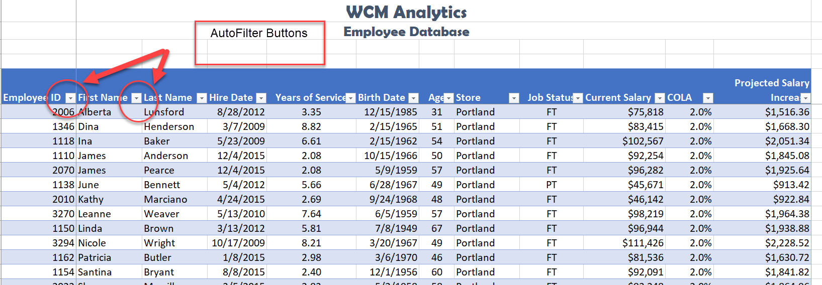
- When you first create a table, Excel automatically enables AutoFilter buttons; a tool used to sort, query, and filter the records in a table. The filter buttons appear to the right of the column headings. When you click the filter button sorting options appear on the menu options.
- From the Home tab, in the Editing group, click the ‘Sort & Filter’ button, and then click one of the sorting options on the Sort & Filter menu.

- From the Data tab, use the ‘Sort A to Z’ or ‘Sort Z to A’ buttons or for multiple levels select the Sort button to open the Custom Sort dialogue.

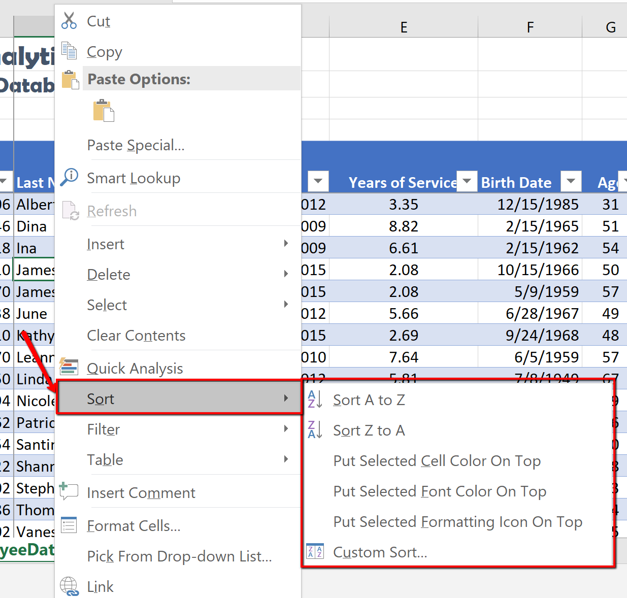
- Right-click anywhere in a table and then point to Sort on the shortcut menu to display the Sort sub-menu.
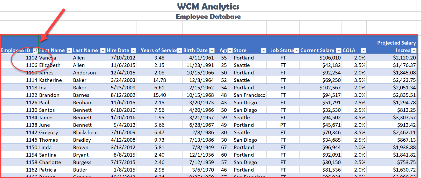
Complete a single level sort by following the steps:
1. In the EmployeeID heading, click the filter button.
2. Choose to Sort Smallest to Largest.
Notice Excel arranges in chronological order all the employee data based on the EmployeeID number, however keeping each record together. You will also notice the filter button now displays an up arrow denoting an ascending sort.
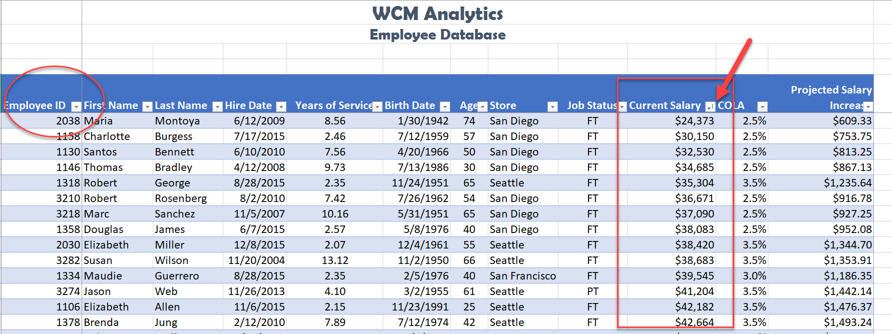
The following steps will sort the records in descending order by Current Salary using the ‘Sort Largest to Smallest’ option form the filter button.
1. Click the filter button located in the Current Salary heading.
2. Choose Sort Largest to Smallest option from the menu.
Notice the original sort has been overridden, and the information is now organized based on the largest Current Salary. You will see the small arrow on the EmployeeID filter is gone, and an arrow pointing down for Descending Order is visible on the Current Salary filter button.
Skill Refreshed
Sort a Column
- Click on the filter Click arrow to the right of the header in the column you want to sort.
- Click on the choice AZ ↑ or ZA↓ to sort your data by that column.
CUSTOM SORT
When you need to sort by more than one level, you must use the Custom Sort option. Complete the following steps to organize the data by Store, Last Name, Current Salary, all in Ascending Order (A-Z).
1. Select the Data tab, and click the Sort button. Notice the last column sorted by is listed. Change the column heading name by dropping down the Sort by menu and select Store.
2. Click Add Level.
3. Click the down arrow in the Then by section, and choose the column heading names as shown below in Figure 5.29 . Note to click Add Level to add the next column heading. The order you select the headings will determine how the table information is sorted.
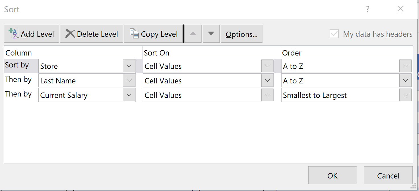
4. Once you select to Sort by column headings, choose the Order by selecting to sort in ascending order (A-Z) for the Store and Last name fields, and Smallest to Largest, for the Current Salary field.
5. Click OK.
Notice the information is now sorted by three levels, per Store , each employee is organized by Last Name , and Current Salary in ascending order (smallest to largest). Each of the filter buttons indicates the sort with the up arrow.
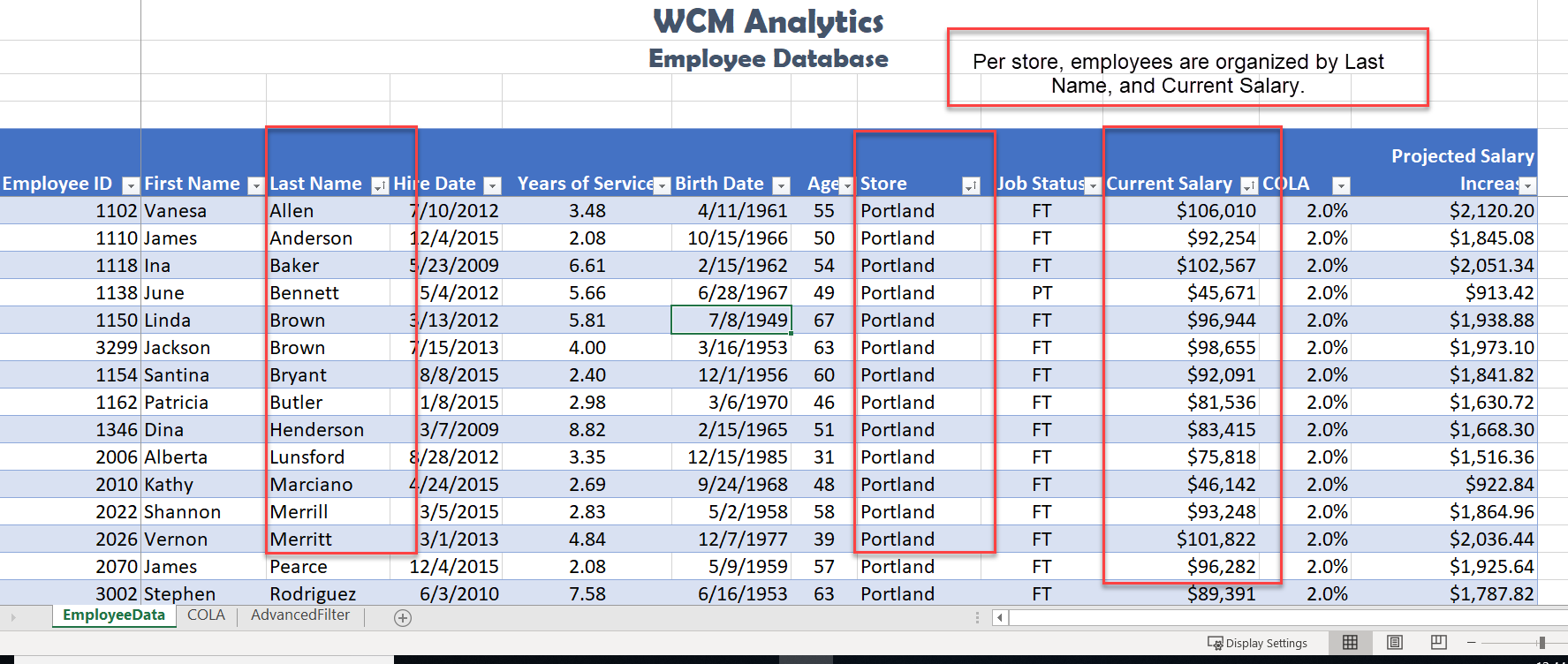
Skill Refresher
Custom Sort (Multiple Level Sort)
- Select the Data tab, and click the Sort button.
- Choose Add Level.
- Click the down arrow in the Column field and choose the column heading to sort by.
- Repeat the above steps to add another level and select the next column heading to sort by.
- The order you select the headings will determine how the table information is sorted.
CUSTOM LIST SORT
When sorting you can create custom lists that allow sorting by characteristics that do not sort alphabetically. Example, text items such as high, medium, and low—or S, M, L, XL. Dates commonly require custom lists so you can vary in the way data is sorted by days of the week or months of the year.
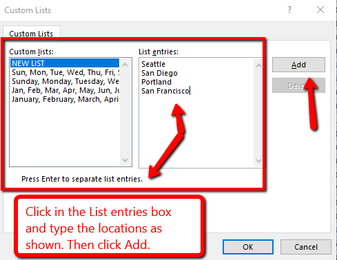
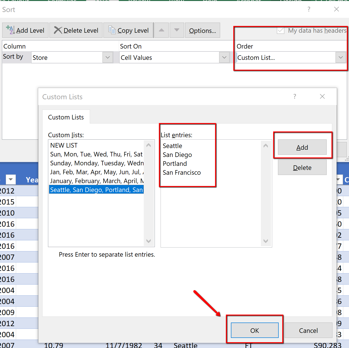
In our case, we want to create a custom list that sorts our stores, which is not, in ascending or descending order. The human resources office likes to order the stores based on the location size. The company headquarters is in Seattle and employs the most people. The next biggest location is San Diego etc. Follow the below steps to create a custom list ordering the stores as shown below:
San Francisco
Follow the below steps to create a custom list ordering:
- While clicked in the table, choose the Data tab and click the Sort button.
- In the Sort by row, click the drop-down menu in the Order Column for the Store heading. Choose Custom List .
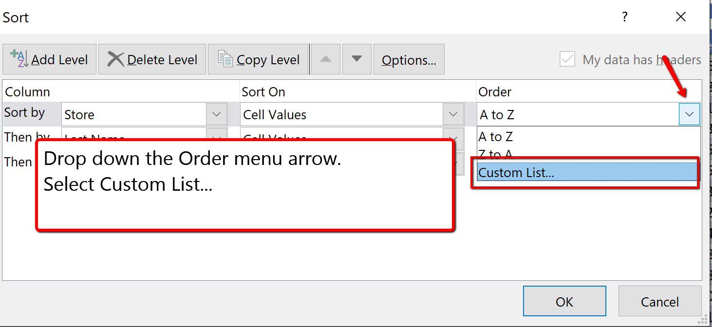
3. Click in the List entries: box and type Seattle , and press enter. Type the remainder of the locations shown in Figure 5.32, pressing enter after each store location typed. Once all locations are entered, click Add . Then choose Ok .
4. You will see the Order of the Store sort update. Click OK to close the Sort dialogue box.

The custom sort is applied and the table is now sorted by Store, using the custom order, then the Last Name of the employee and then by the Current Salary column.
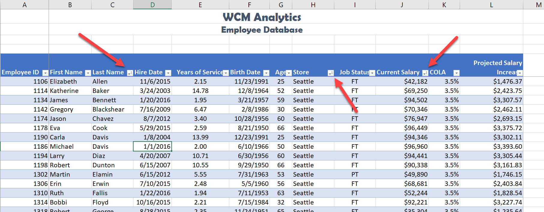
- Click the Excel menu option and choose Preferences
- Type the list of cities in the “List entries” box as shown in Figure 5.32 above then click the Add button and close the Custom List dialog box
- Click anywhere in the table, and then click the Data tab and click the Sort button
- Click the drop-down menu in the Order Column for the Store heading. Choose Custom List
- Click on the custom list of cities that you just created and then click the OK button twice
- The custom sort is applied and the table is now sorted by Store, using the custom order, then the Last Name of the employee and then by the Current Salary column. See Figure 5.34 above.
Custom List Sort
- Click the drop-down menu in the Order Column of the field needing a custom list created.
- Choose Custom List.
- Click in the List entries box and type the custom list desired.
- Then click Add.
FILTER DATA
If your worksheet contains a lot of data, it can be difficult to find information quickly. Applying Filters is an efficient and effective way to only show the information needed. Typically when filtering you are searching the data for specific information. Generally speaking, you are searching the data based on a question, or in other words, querying the data, and returning only the information that satisfies the question. The process of filtering records based on one or more filter criteria is called a query. Filtering data hides the rows whose values do not match the search criteria. The information that does not display is not deleted, it is just hidden, and will be redisplayed by removing the filter or applying a new filter.
Like sorting, Filter options are located in the filter button alongside each field name. By clicking the filter button, you can choose which values in that field to display, hiding the rows or records that do not match that value. The filter lets you choose to display only those records that meet specified criteria such as color, number, or text. In this situation, criteria is defined as; a logical rule by which data is tested and chosen.
For example, you can filter the table to display a specific name or item by typing it in a Search box. The name you selected acts as the criterion for filtering the table, which results in Excel displaying only those records that match the criterion. The selected checkboxes indicate which items will appear in the table. By default, all of the items are selected. If you deselect an item from the filter menu, it is removed from the filter criterion. Excel will not display any record that contains the unchecked item. As with the previous sort techniques, you can include more than one column when you filter by clicking a second filter button and making choices. After you filter data, you can copy, find, edit, format, chart, or print the filtered data without rearranging or moving it.
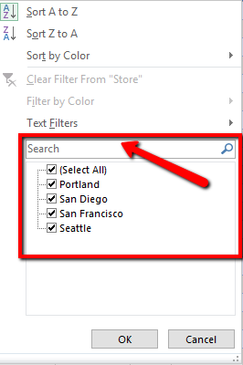
Complete the following steps and filter data according to each query.
How many employees are at a Part-Time (PT) status?
- Click the filter button on the Job Status column heading.
- Click Select All , to deselect options.
- Click the PT box to only display the part-time employees.
- From the total row, in cell I108 , choose the Count function count the number of employees at a PT status.
The answer to the question is there are currently are 11 employees at a PT time status. The total row will display the part-time total current salaries, and what the projected salary increase for part-time help will be after COLA adjustments.

USING CRITERIA FILTERS
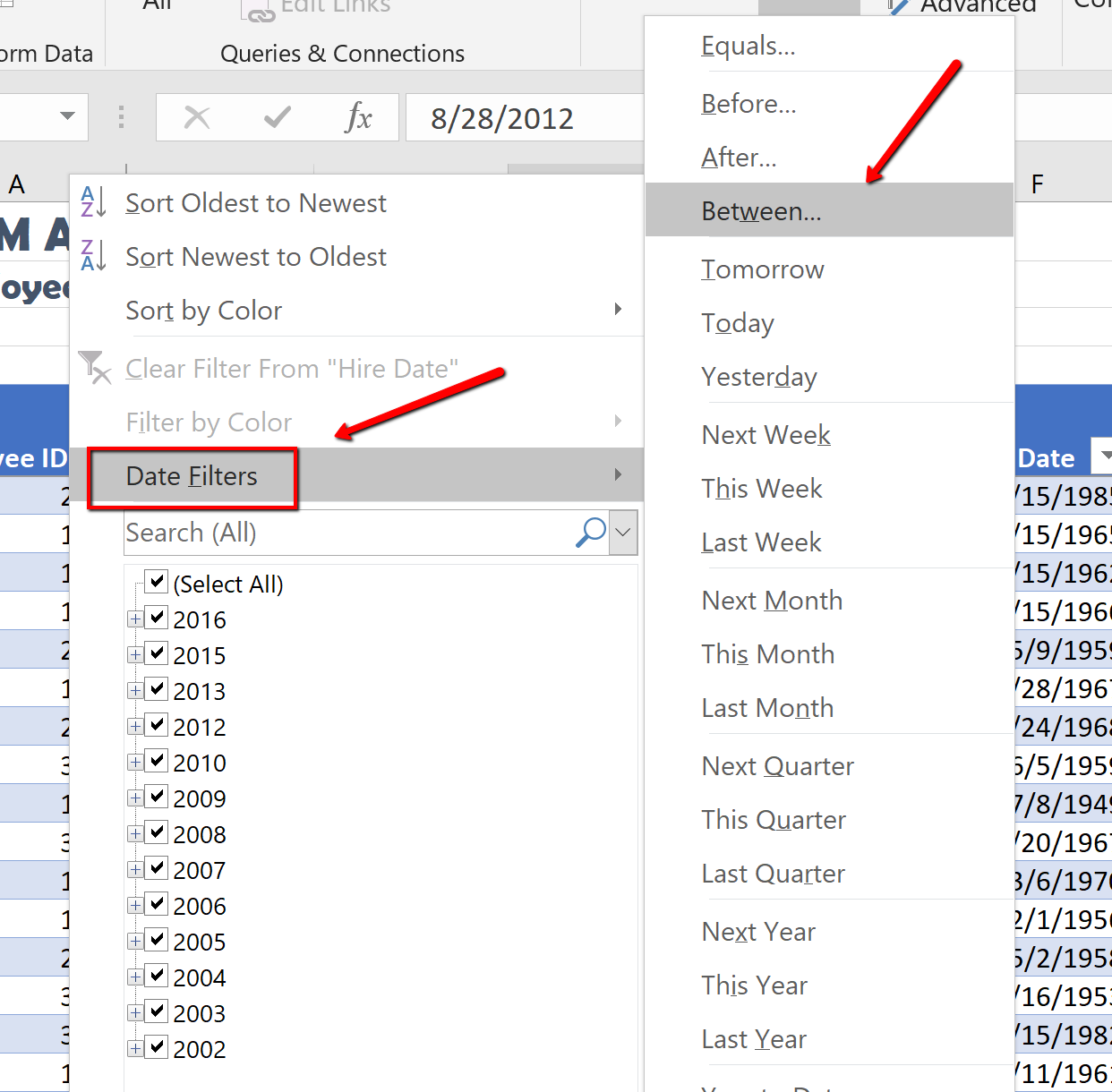
The filters created are limited to selecting records for fields matching a specific value or set of values. For more general criteria, you can use criteria filters, which are expression involving dates and times, numeric values, and text strings. Excel will identify what criteria filter to display based on the information in the column. For example, you can filter the employee data to show only those employees hired within a specific date range. Notice the criteria filter changes to Date Filters. If we were looking at the Current Salary column, the filter would be a Numbers Filter.
Using criteria filters, follow the below steps to search for employees who have been with the company for a specific time period.
Identify employees who have been with the company between 2013-2016.
2. Click the Filter button in the Hire Date column. Select Date Filters, and choose the Between criteria.
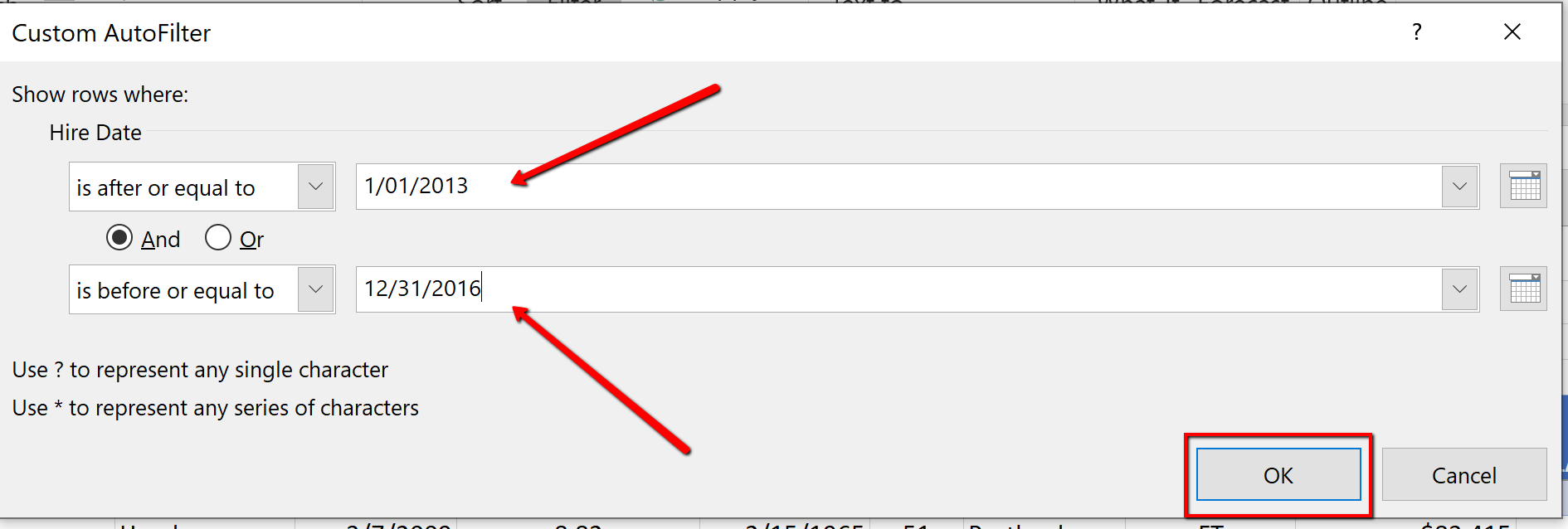
3. Search for employees with a hire date between 2013, and 2016. In the “ is after or equal to” section type 1/01/2013 , and typing in the “ is before or equal to” section type 12/31/2016 . Then click OK .
4. Sort the filtered table from Oldest to Newest by Date Hired.
5. In the total row section, count the last name names of the employees by applying the count function in cell B108.
6. In the total row, select cell I108 , and choose None to turn off the count function in the Job Status Column.
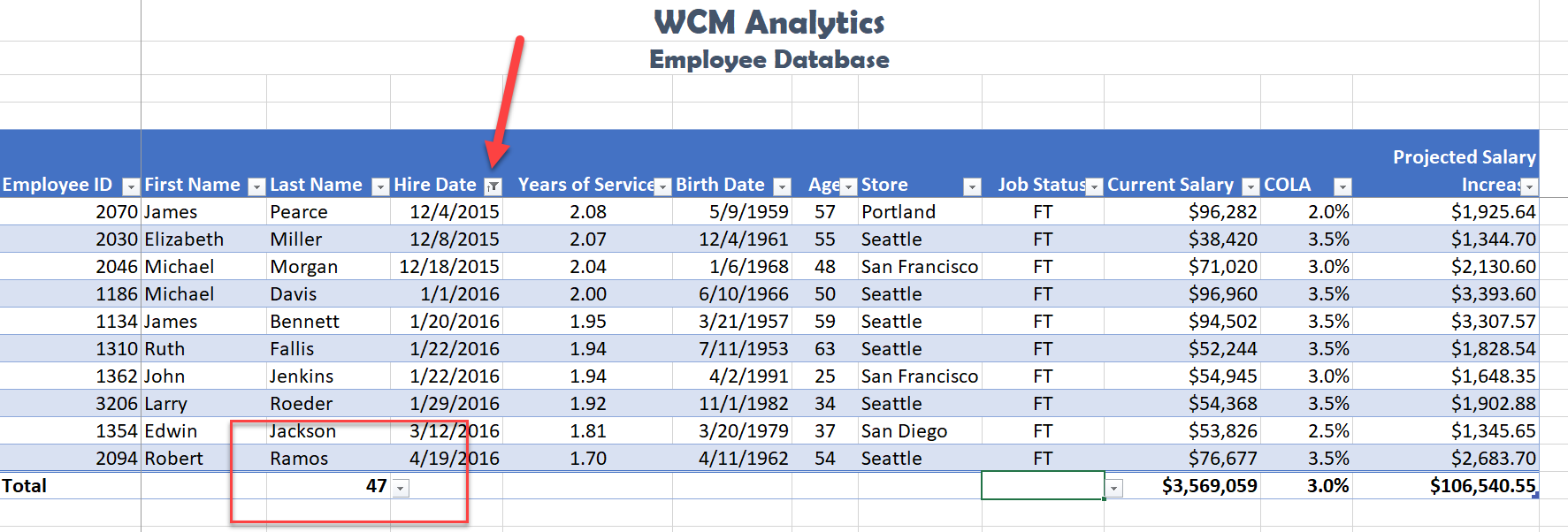
Notice the table total row show 47 employees hired between the specified dates. These employees will be evaluated for a COLA adjustment.
Notice the filter button displays a filter symbol and an up arrow indicating the column is filtered and sorted in ascending order.
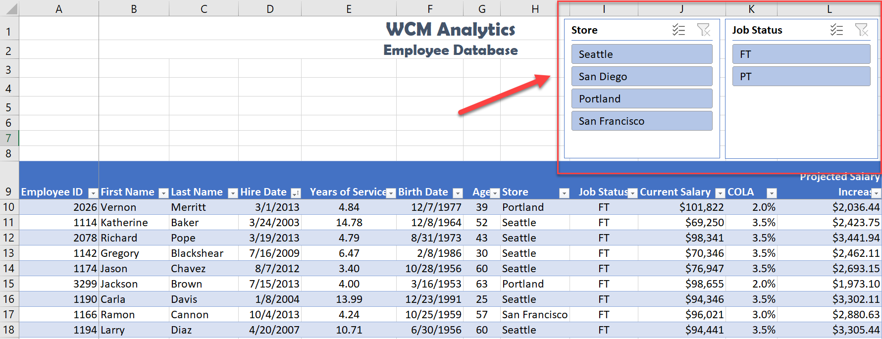
Another way to filter an Excel table is with slicers. Slicers, generally speaking, are visual filter buttons you can click to filter the table data. Slicers show the current filtered category, which makes it easy to understand what exactly is displayed. For example, a slicer for the Store field would have buttons for the Seattle, San Diego, Portland, and San Francisco locations.
When slicer buttons are selected, the data is filtered to show only those records that match the criteria. Multiple buttons can be selected at the same time, and a table can have multiple slicers, each linked to a different field. When multiple slicers are used, Excel uses the AND logical operator so filtered records must meet all of the criteria indicated in the slicer. When selecting multiple buttons in a Slicer, use the shift key to select adjacent field names. If the field names are not adjacent, use the non-adjacent selection method, pressing the CTL button, and selecting the field names needed.
Follow the below steps to filter the table using visual Slicer buttons.
1. Click in the table area. From the Data tab, choose Clear to remove the current sort and filter applied to the data.
2. To make room for the Slicer buttons at the top of the table, we will add 4 rows between the title and the table area. Right-click cell A3. Choose Insert. Select Entire Row . Repeat these steps until the table heading starts in row A9 .
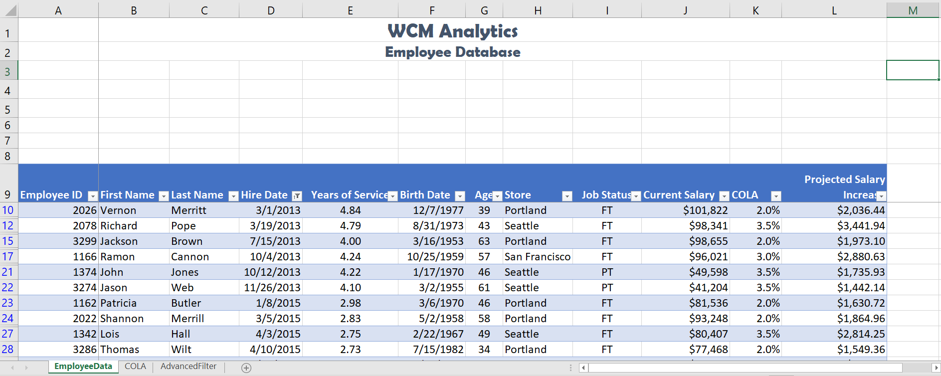
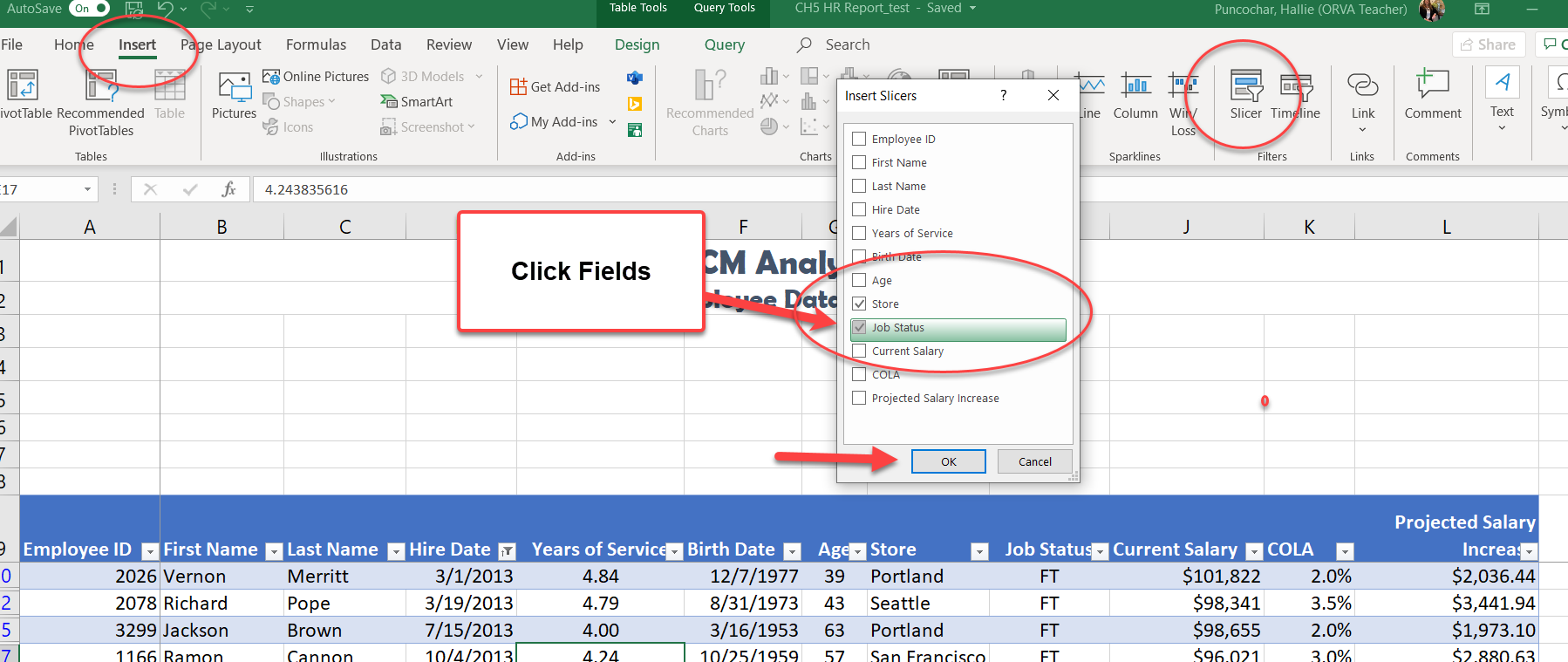
3. Click back into the table area. Choose the Insert tab. Click Slicer . When the Insert Slicers dialogue box opens, click the Store and Job Status field names to display as slicers. Click OK .
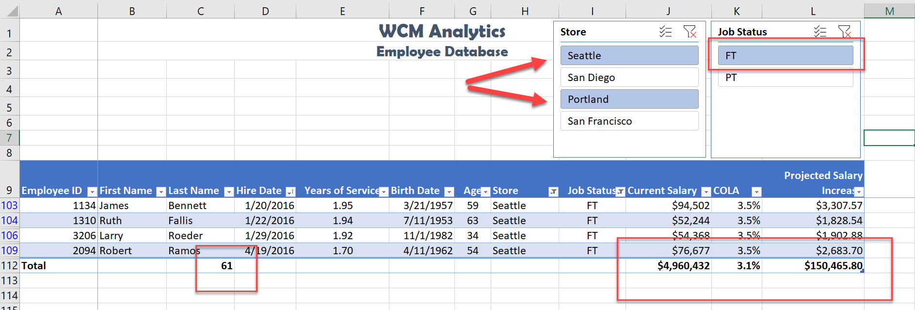
4. Move, and re-size the Slicer boxes to fit in the approximate area of I1:J8 and K1:L8 . Make sure the buttons remain visible. Below is a visual example.
5. From the Store slicer, click the San Diego button. Notice the data filters to only show the data for San Diego.
6. From the Job Status slicer click PT . Notice the data filters to only show the data for PT employees in San Diego.

8. Change the Job Status slicer selection to FT .
The table results show there are 61 FT employees in Seattle and Portland. The Projected Salary Increase after the COLA adjustment for the Northwest region is $150,465.80.
ADVANCED FILTERS
Filter buttons are limited to combining fields using advanced logic or complex criteria. If the data you want to filter requires complex criteria, you can use the Advanced Filter dialog box. The Advanced Filter works differently from the Filter command in several important ways:
- It displays the Advanced Filter dialog box instead of the AutoFilter menu.
- You type the advanced criteria in a separate criteria range in a worksheet and above the range of cells or table that you want to filter. Excel uses the separate criteria range in the Advanced Filter dialog box as the source for the advanced criteria.
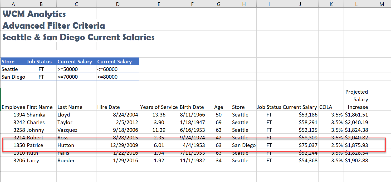
For example, you searched records for employees in the Seattle and San Diego offices AND for employees working at full-time bases, AND have a base salary between the below Salary Ranges:

To run the above complex criteria mentioned above follow the below steps:
- From the EmployeeData sheet, click in the table, then select the Data tab and clear the current filters by selecting the Clear button.
- Select the Advanced Filter sheet. Click cell A10. The criteria mentioned in the above example has already been entered for this advanced filter exercise. Next, you will use an advanced filter to copy the records that match these criteria.
- From the Data tab, click the Advanced button. The Advanced Filter dialog box opens.
- Click the Copy to another location option button to copy matching records from the data range.
- Click, or press the tab key, to move to the Criteria Range box.
- From the Advanced Filter sheet, select A6:D8. You will see ‘Advanced Filter’!Criteria populate in the criteria range box.
- Click, or press the tab key, to move to the Copy to box, and then click cell A10 to specify the location for inserting the copied records. You will see ‘Advanced Filter’!$A$10 in the Copy to criteria range box.
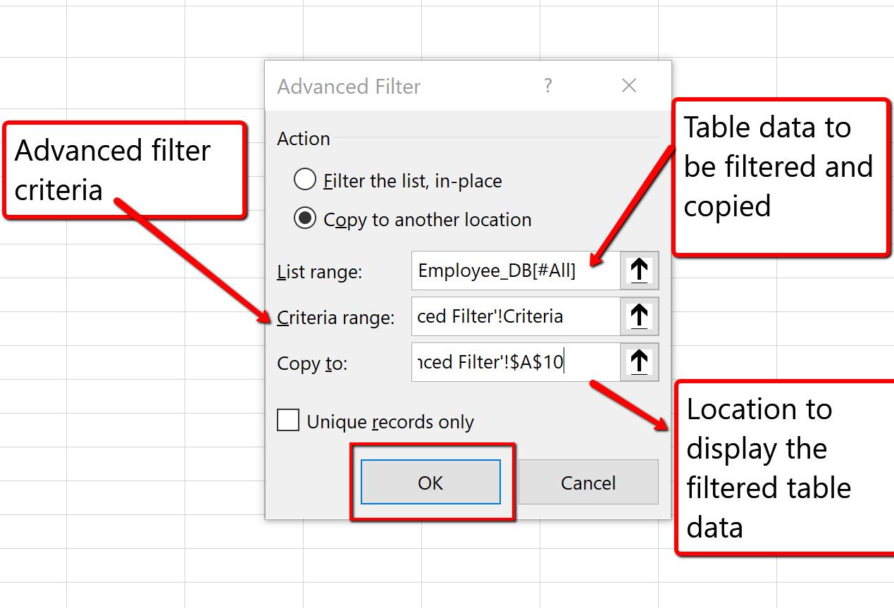
9. Click OK to copy the records that match the advanced filter criteria. Save your work.
The advanced search results list 7 employees that meet the criteria. Of these 7 employees, only 1 full-time employee in San Diego has a current salary between $70,000 and $80,000 dollars, and 6 full-time Seattle employees have a current salary between $50,000 and $60,000 dollars.
INSERT TABLE
Let’s review another away to turn a range of data into a table.
- Select the Advanced Filter sheet, and click cell A10.
- From the Insert tab, choose Table .
- The Create Table dialogue box will appear.
- Make sure “My table has headers” is selected so Excel recognizes the column headings.
- Click OK . Excel turns our advance search data into a table.
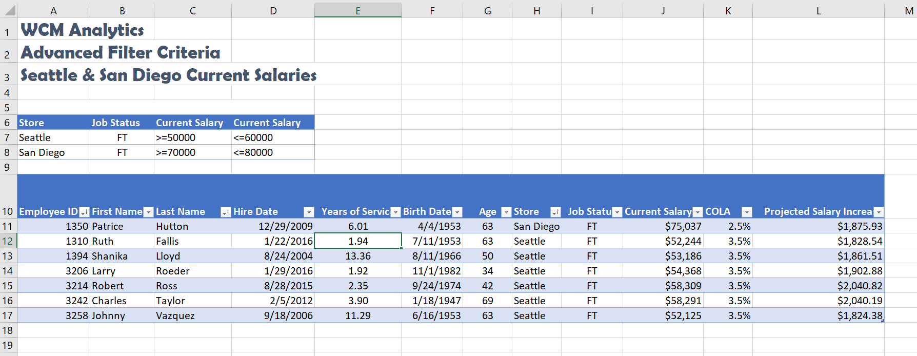
- Sort the table in ascending order (A-Z), by Store, and Employee ID, then Last Name. Hint: Click the Data tab, Click the Sort button, add levels for the three fields.
- Autofit the column widths and row height to make sure the heading row is visible.
- Save your work.
Excel turns the information into a table and sorts accordingly:
ANALYZING WORKSHEET DATA
INTRODUCTION TO PIVOT TABLES
Another way to analyze table information is with PivotTables. A PivotTable is a powerful tool that calculates, summarizes, and analyzes table data to compare, patterns, and trends. PivotTables are inserted directly from a table, linking the table data. Generally speaking, when you pivot on the table data you are reorganizing the table information to reveal different levels of detail that allow you to analyze specific subgroups of information and summarize data quickly and easily without having to change the structure or layout of the original table area.
When you pull table data into a PivotTable there are four main area fields: Rows, Columns, Values, and Filters. The Rows and Columns fields can interchange quickly to summarize the data in different ways or to run new reports based on the question or criteria being asked. The Value field is data from the table that can be calculated, or that contain values that the PivotTable will summarize. The Values field has multiple settings to choose how you want to calculate the data; SUM, COUNT, AVERAGE, MIN, MAX, and can even show the displayed values as a percentage of the total, column total, grand total, and so on. Lastly, is the Filters area, which restricts the PivotTable to only show the values matching specified criteria.
Four Primary PivotTable Areas:
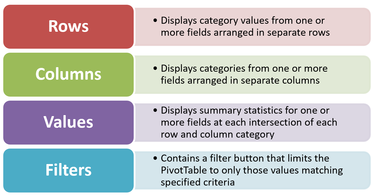
Figure 5.49 Four Primary PivotTable Areas
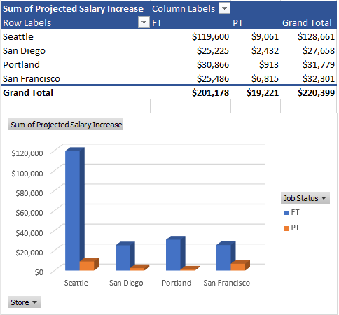
In our situation, shown below, we will create a PivotTable to summarize employee data to show Projected Salary Increases, for both Part-Time (PT) and Full -Time (FT) employees for all store locations.
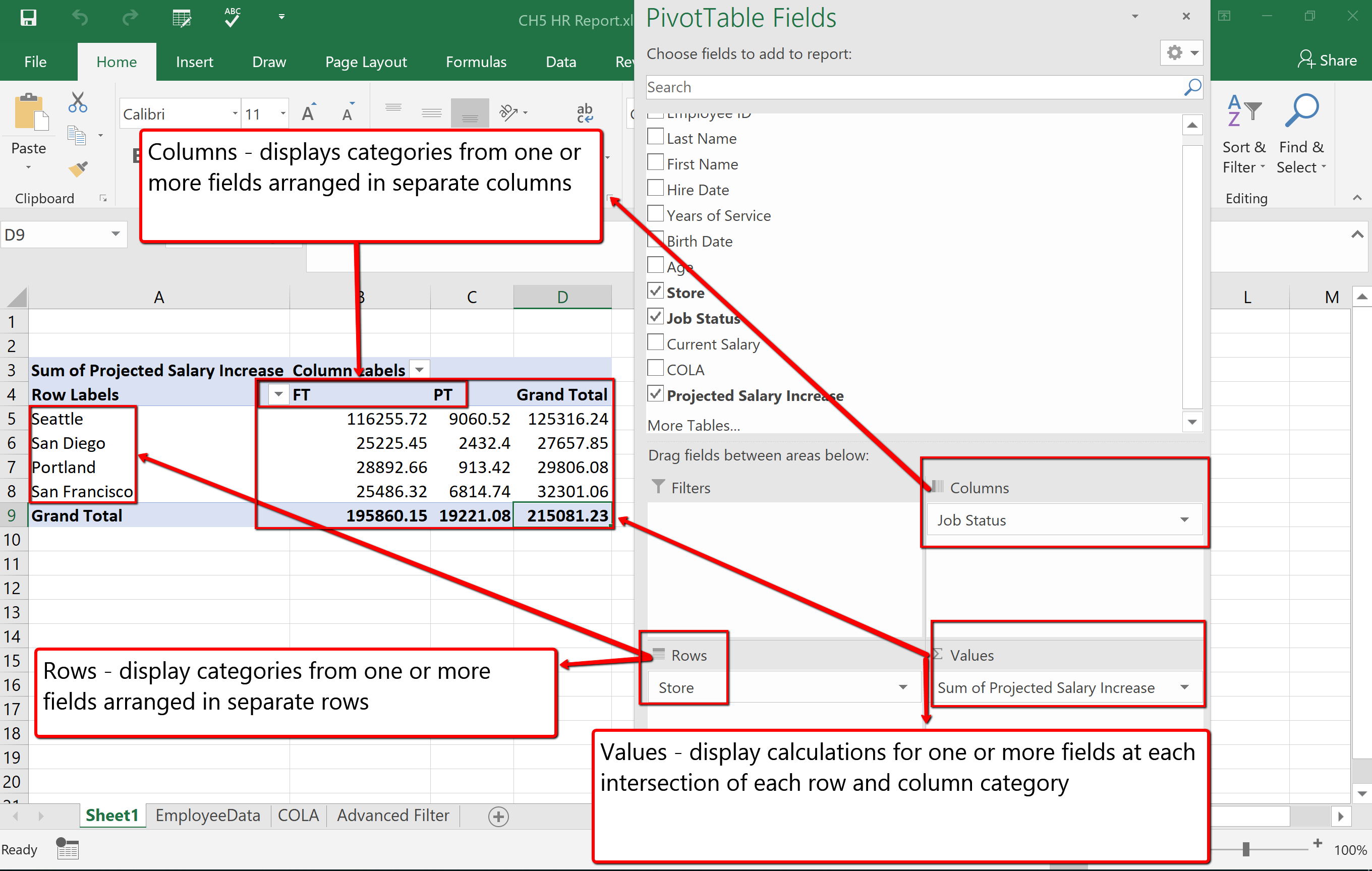
Follow the below steps to explore and build a PivotTable report.
- Click the EmployeeData sheet. Click anywhere in the table area.
- From the Insert tab, choose PivotTable .
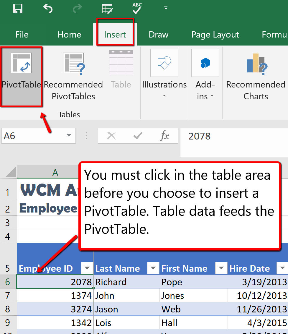
3. From the Create PivotTable dialogue box, make sure the PivotTable report will be placed in a New Worksheet , and click OK .
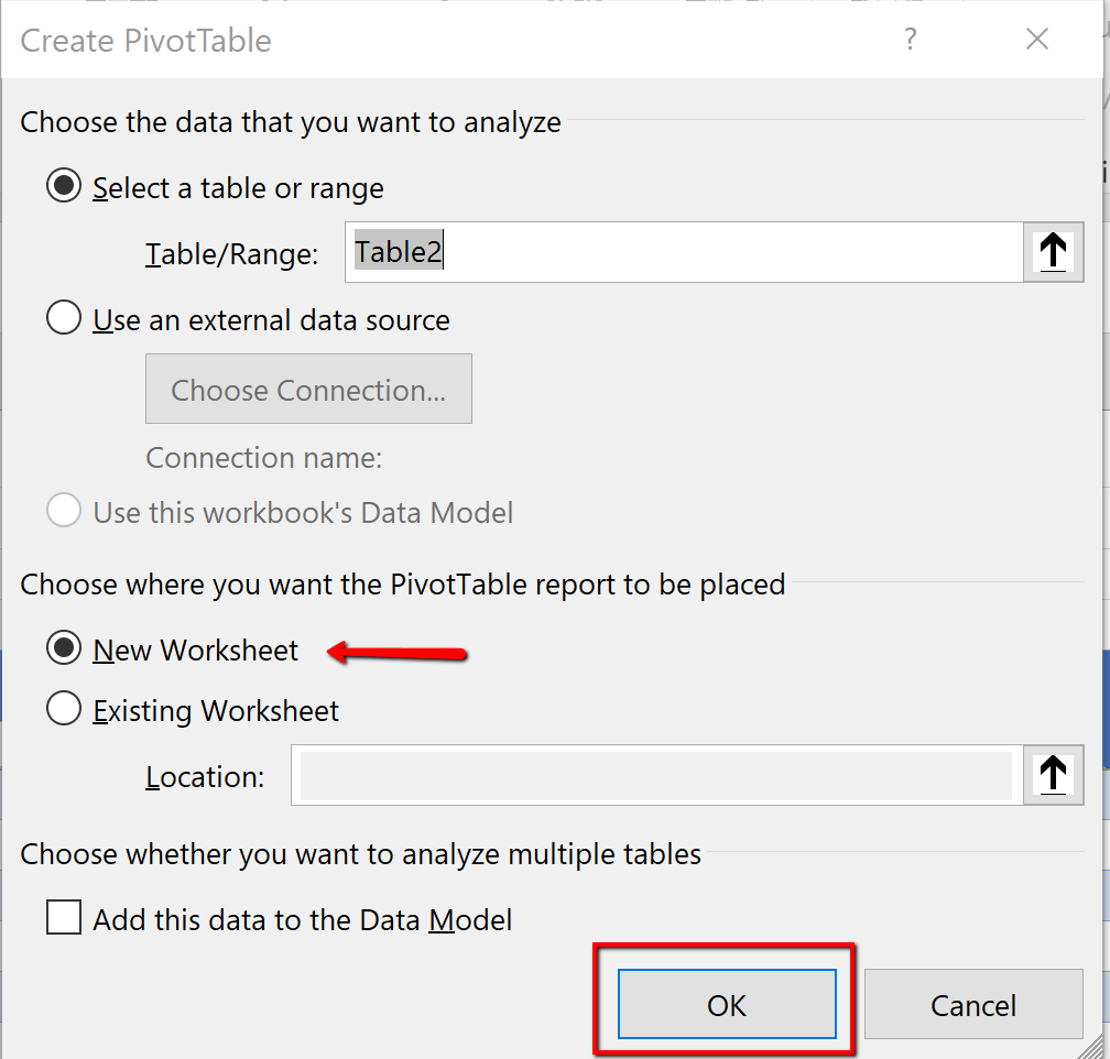
4. Notice a new sheet (Sheet1) is inserted, at the bottom of the workbook, that contains the PivotTable1 area and fields dialogue box. Rename the default name (Sheet 1) to StorePT .
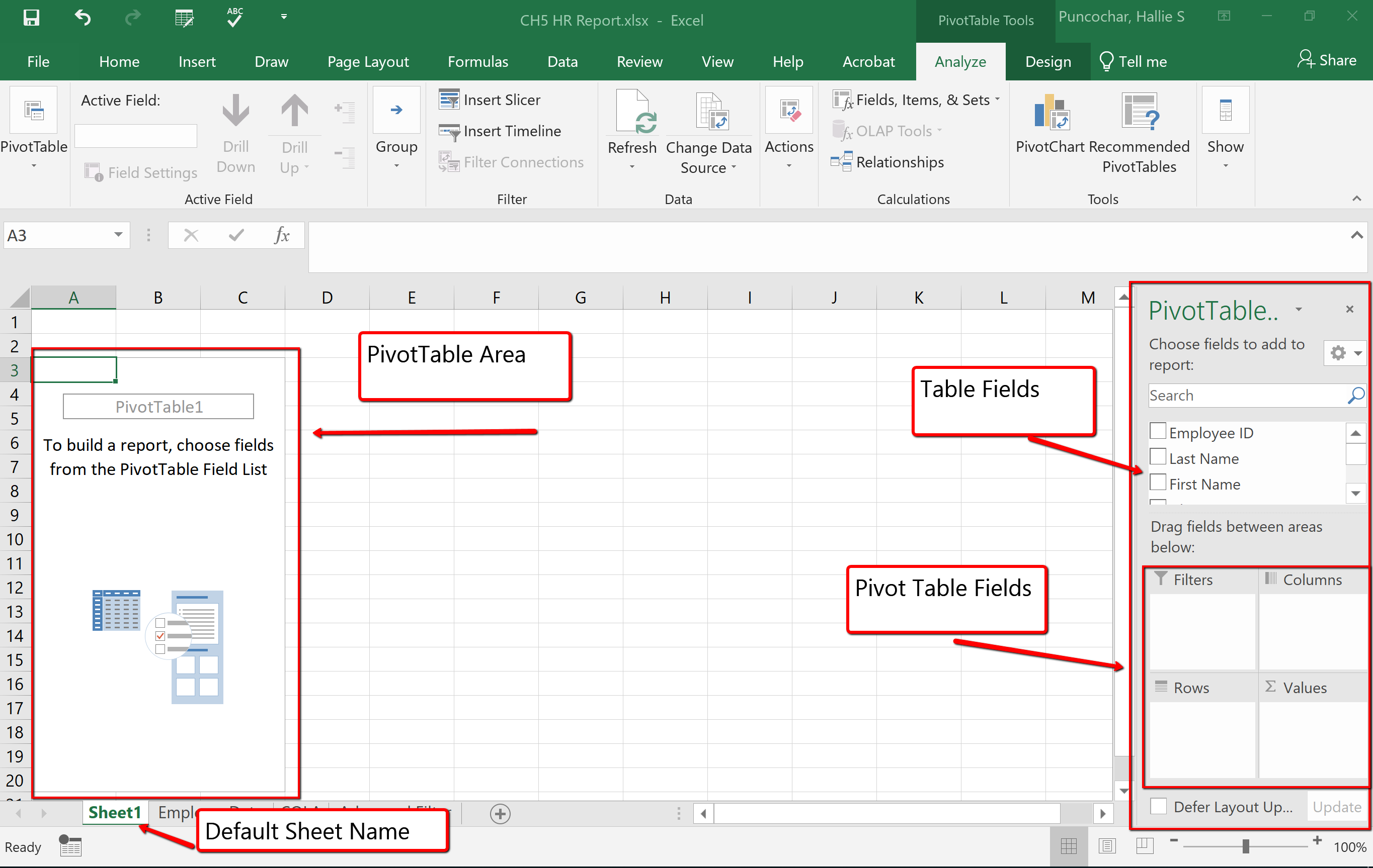
5. From the PivotTable pane, drag and drop the Store heading to the Rows section of PivotTable field area.
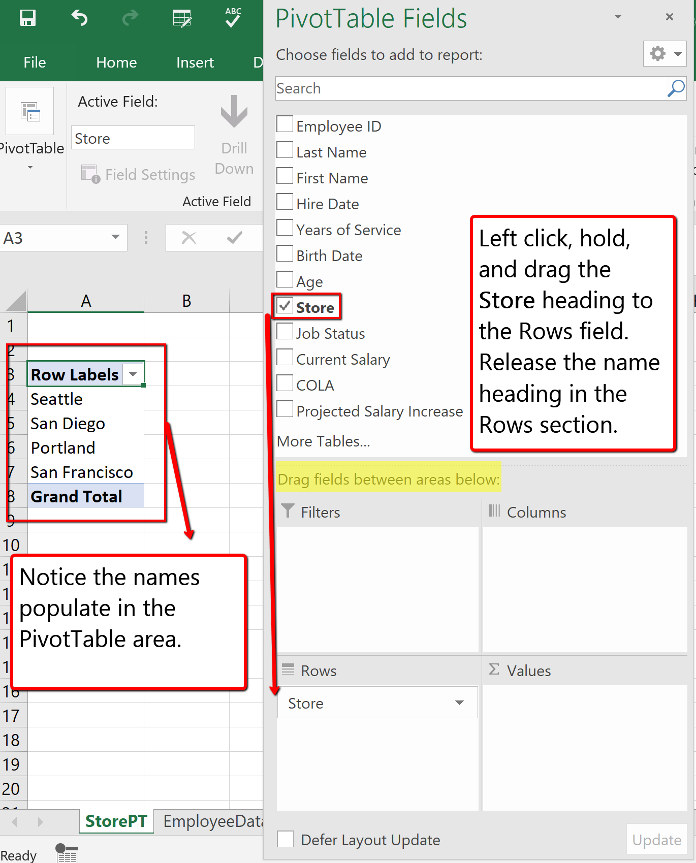
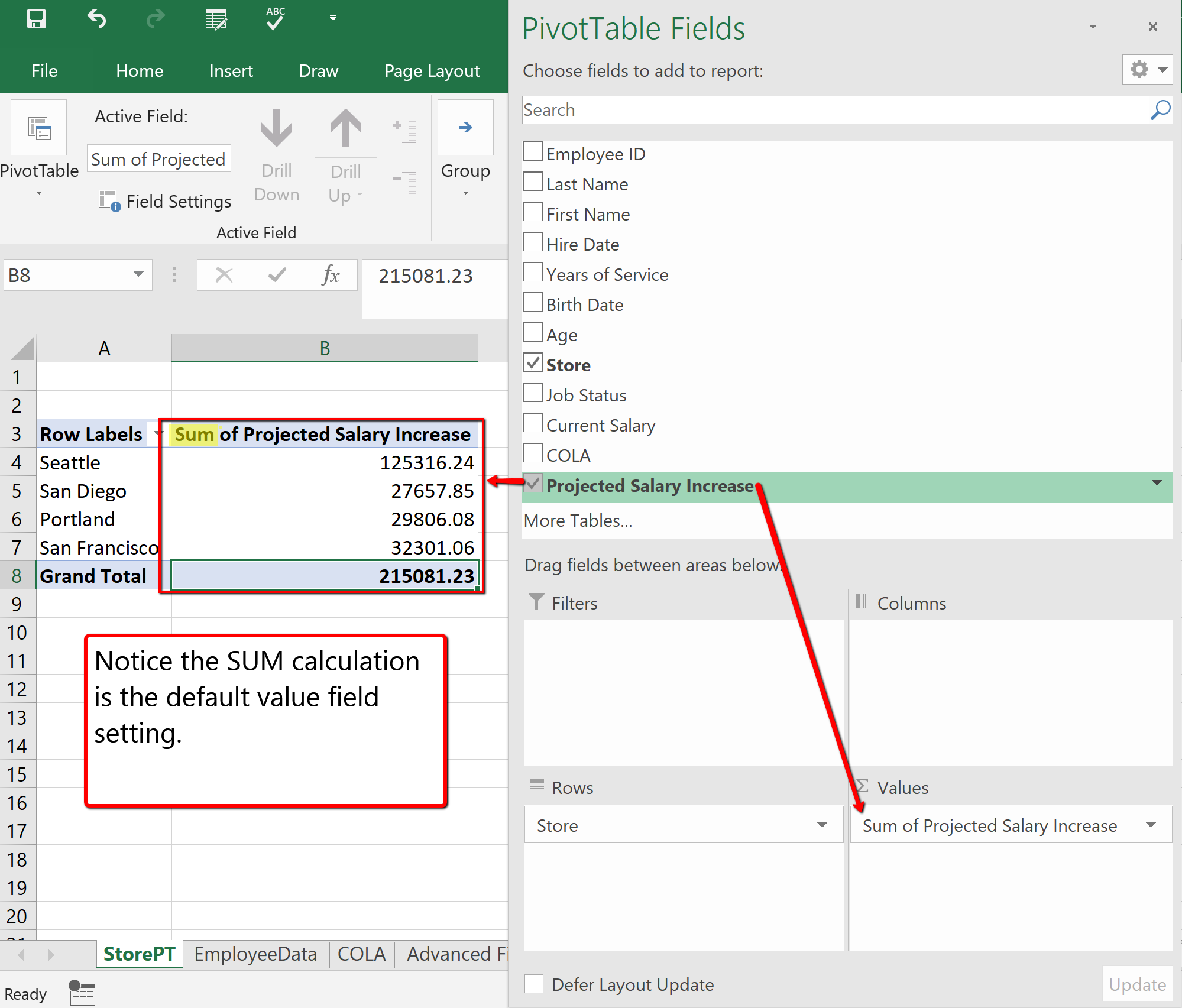
6. From the PivotTable fields list drag and drop the Projected Salary Increase heading to the Values section.
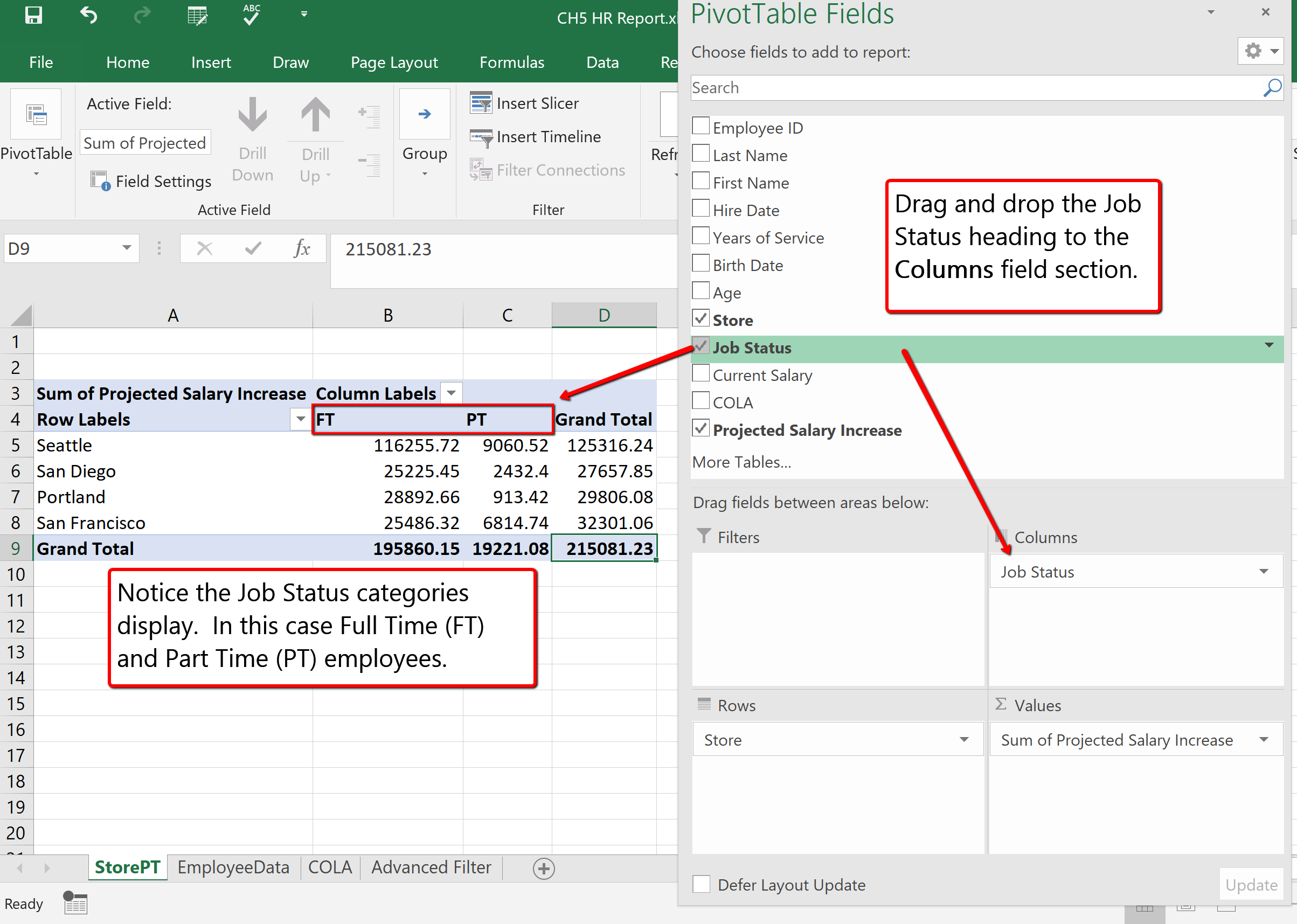
7. Drag and Drop the Job Status heading to the Columns field section. Notice the Job Status categories display. In this case, displaying Full-Time (FT) and Part-Time (PT) employees.
FORMATTING PIVOT TABLES
The Analyze tab contains tools specifically for examining data, for example, the ability to insert Slicers, or PivotCharts. The Design tab contains tools that specifically tie to how the table and data visibly display. For example, when you have a lot of data in your PivotTable, it may help to show banded rows or columns for easy scanning or to highlight important data to make it stand out.
Follow the below steps to add format the PivotTable, and add a PivotChart.
- Click in the PivotTable. From the PivotTable Tools choose the Design tab.
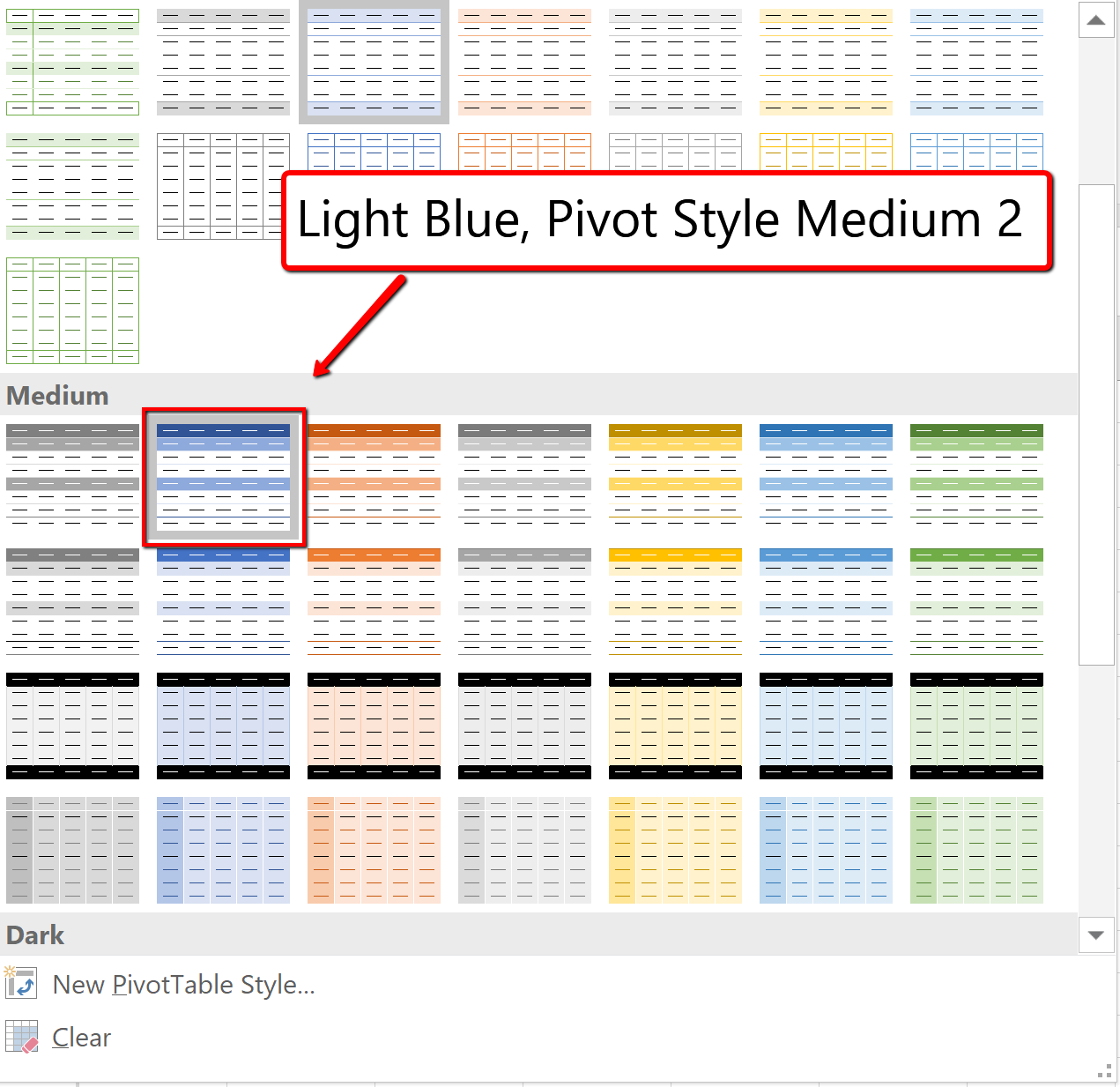
- In the PivotTable Styles gallery select the Light Blue, Pivot Style Medium Style 2 format.
3. To format the PivotTable numbers, select B5: D9. Click the Home tab. Apply the Currency number format and decrease the decimal place to zero decimals.
NOW LET’S CREATE A PIVOTCHART !
4. Click in the PivotTable. Click the Analyze tab. Choose the PivotChart button on the Ribbon.
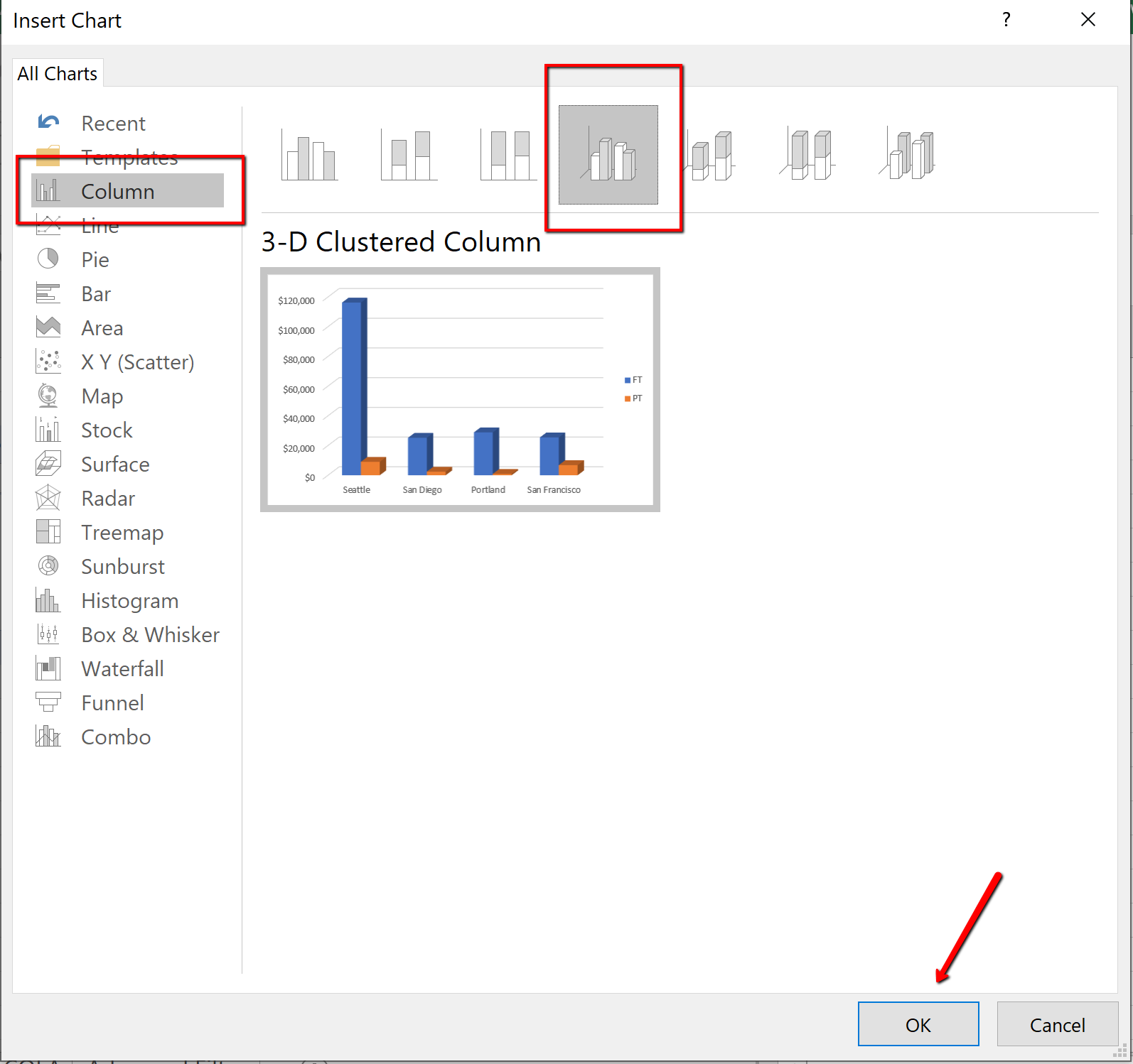
5. From the listed chart types, choose Column. And select the 3D Clustered Column option. Click OK.
- Click on the 2D chart that was just inserted
- Click the Design tab on the Ribbon
- Click the Change Chart Type button
- Select the 3D Clustered Column option
6. Move the PivotChart under the PivotTable area. Resize accordingly. Save your work.
Note the formatting changes in the new chart below. The “Job Status” and “Store” buttons are column and row “filters” for the Pivot Chart.
Another way to summarize data is by using subtotals. Analyzing a large data range usually includes making calculations on the data. You can summarize the data by applying summary functions such as COUNT, SUM, and AVERAGE to the entire organized range of information. Subtotals, in general, are summary functions applied to parts of an organized data range.
For example, you can SUM Current Salaries for employees from each Store location. To subtotal the information the data must first be sorted by the Store field. For subtotals, the field that you sort is referred to as the control field. For example, if you choose the Store location as your control field, all of the Seattle, San Diego, Portland, and San Francisco entries will be grouped together within the data range. The SUM function then can be applied to SUM the Current Salary fields for each Store location. Excel calculates and displays the subtotal each time the Store location changes.
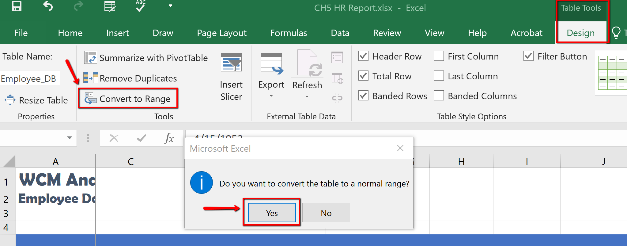
A new row containing a subtotal of that particular location will be inserted, and wherever the field changes a value will display; a subtotal group of records. Excel updates the subtotal automatically when the control field is changed. In theory, when subtotaling, you are adding a calculation row to the set of data. Adding rows that total information in the middle of a table would compromise the integrity of data in the table. The table tools would look at the total as a record, not a calculation. Therefore the Subtotal feature cannot be used in tabling, and can only be applied to a normal range of data. You must convert all tables to a range prior to subtotaling.
Multiple functions can be applied within the same Subtotal. For example, we will explore how you can SUM Current Salary’s and also provide the AVERAGE Current Salary for each Store location within the same Subtotal. Note Subtotal data can also be filtered.
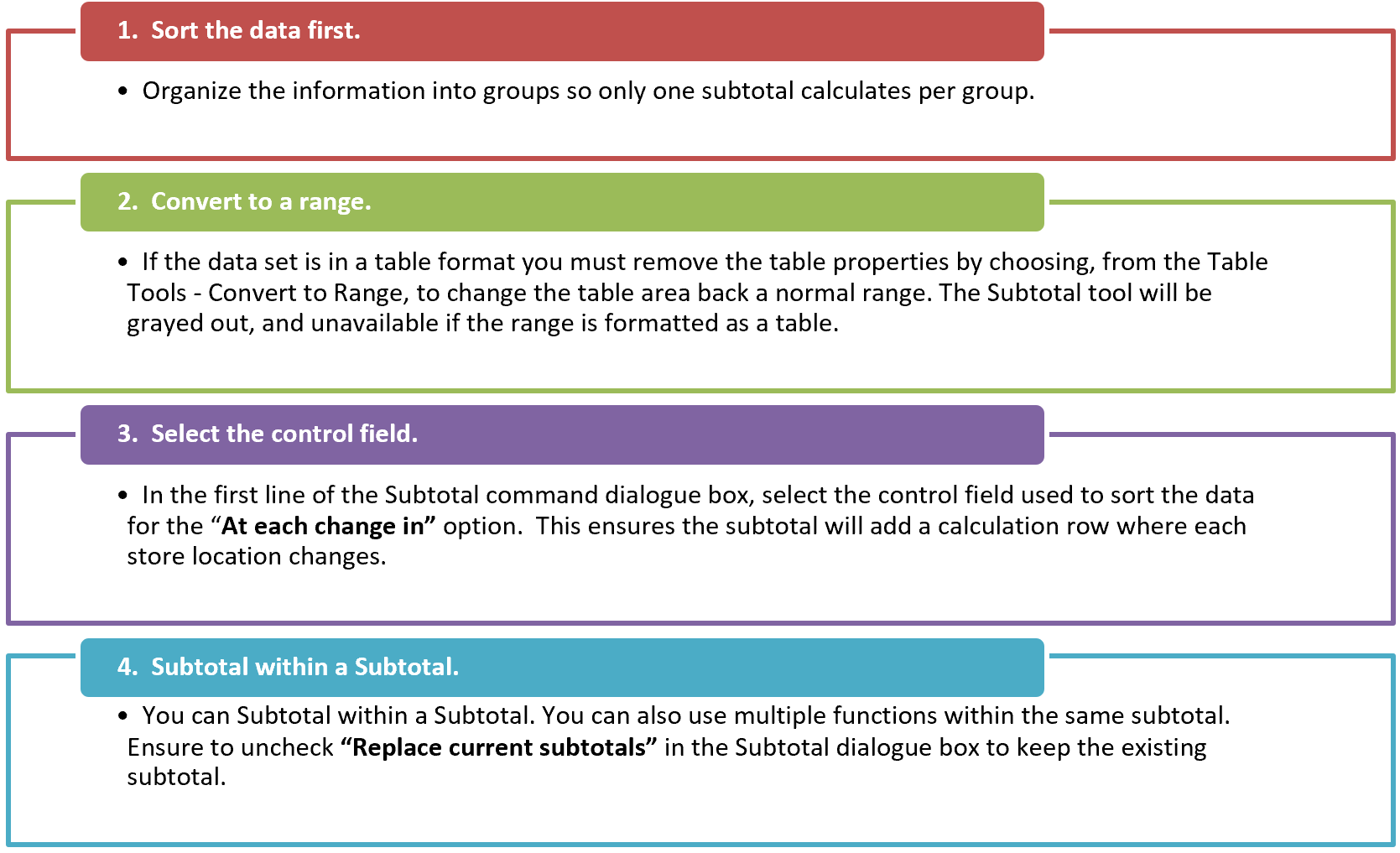
The best practice when subtotaling is to follow four rules:
Follow the below steps to Subtotal the Employee Data and provide a total Current Salary per Store.
- Select the Employee Data sheet. If necessary clear any filters applied to the data by clicking the Data tab and choosing the Clear filter option.
- From the Data tab, choose Sort button. Sort the Store Location, using the preferred Custom List order of Seattle, San Diego, Portland, and San Francisco. If the list we set up previously is not available type the entries in the List entries area. Choose Add, and then OK.
Select “ Convert to Range .” Excel will display a message asking if you really want to convert the table back to a normal range. Choose Yes.
4. Click the Data tab, in the Outline group find and select the Subtotal Command. (Notice the heading row no longer has filters buttons. The data looks like a table but is not a table. The table tools are not active, and the information is a normal range.)
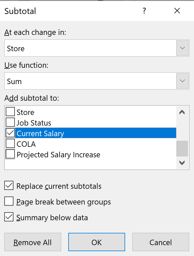
5. In the Subtotal dialogue box, choose the Store field in the “ At each change in .” For the “ Use Function ,” choose Sum , and only check Current Salary . Click OK.
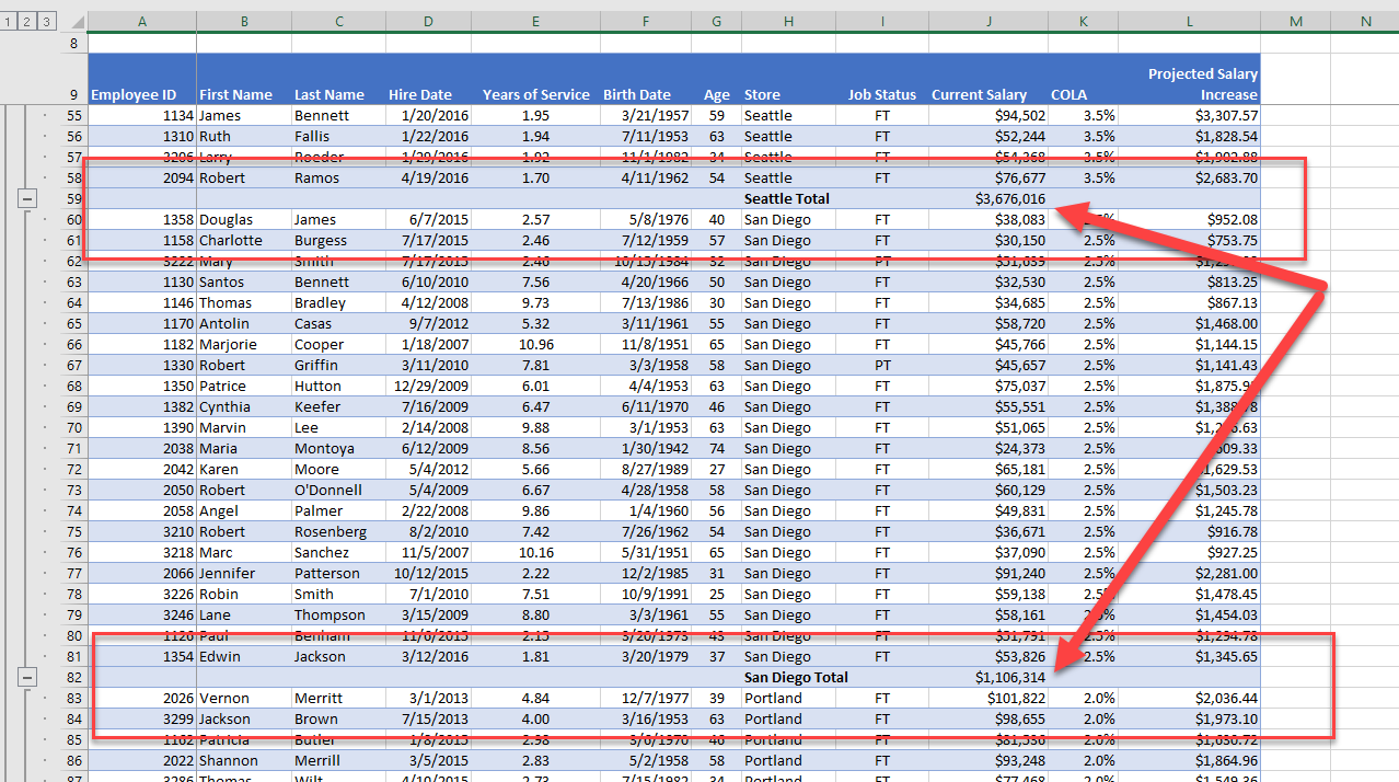
6. Notice the Current Salary column is totaled, per location. Save your work.
SUBTOTAL OUTLINE VIEW
The Outline views, located on the left side panel, show summary statistics. The Outline tool, with levels, allows you to control the expanse of detail displayed in the worksheet. The EmployeeData worksheet has three levels in the outline of its data range:
- Level 1, displays only the grand totals.
- Level 2, displays the total spent at each Store.
- Level 3, displays the total Salary.
Figure 5.66 above shows the Level 3 Outline, all the employee detail per store location. Clicking the outline buttons located to the left of the row numbers lets you choose how much detail you want to see in the worksheet. (Note that the three level numbers are at the top left side of the worksheet, just below the Name box.)
You will use the outline buttons to expand and collapse different sections of the data range.
- Click level 1. Notice it displays the Grand Total.
- Click level 2. Notice the totals for all store locations are displayed.

ADDING A SUBTOTAL WITHIN A SUBTOTAL
As mentioned at the beginning of the section, you can use multiple functions within the same subtotal. We will now explore how you can SUM Current Salary’s and also provide the Average Current Salary for each Store location within the same Subtotal.
- Click within the Subtotal data, go to the Outline, click Level 3, to display all the subtotal data.
- From the Data tab, and click Subtotal.
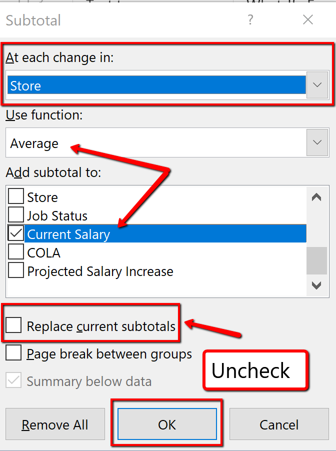
- In the Subtotal dialogue box, select the Store field for the “ At each change in:” option.
- In the “ Use function:” section select to display the Average .
- Only check the Current Salary field in the “Add subtotal to section:” . (Note Excel will default check something in this area. Uncheck any other fields.)
- Uncheck “Replace current subtotals” ; we do not want to replace the current subtotal summing the Current Salary.
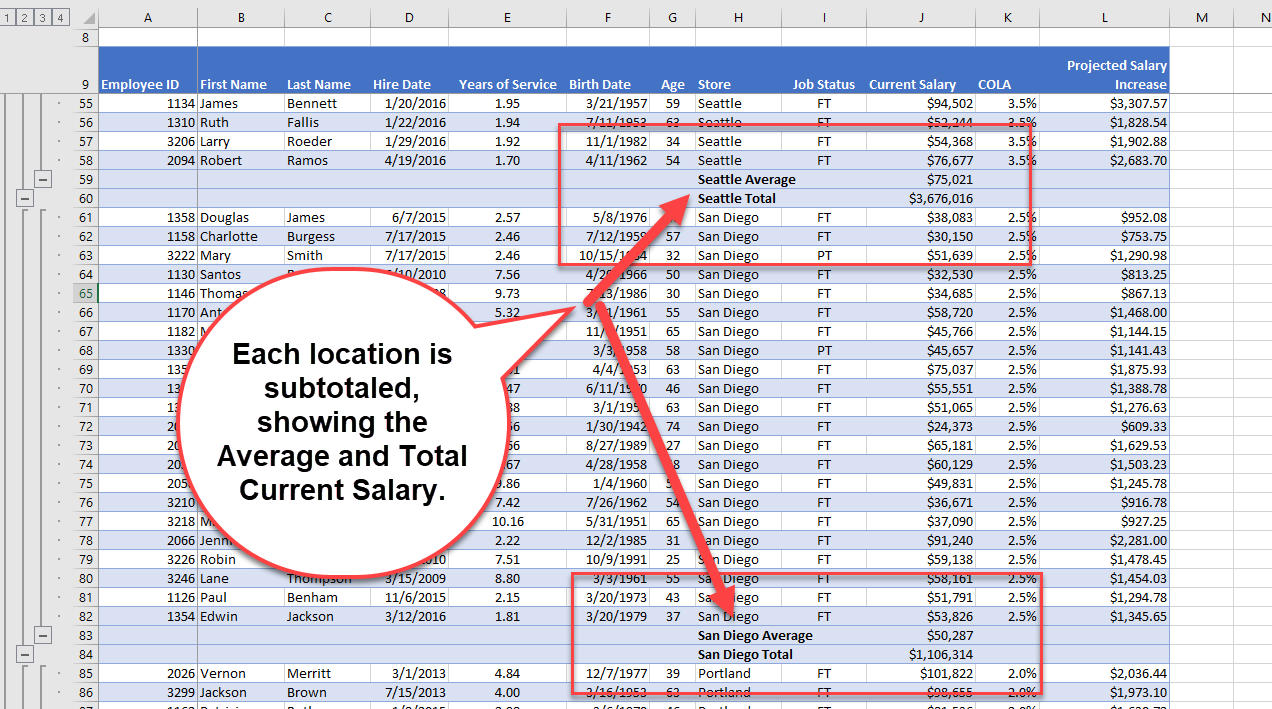
8. Notice each location is now subtotaled showing the Average and Total Current Salary. Excel has also added 4th level to the Outline, accounting for the Averages. Save your work.
Key Takeaways
- A table is made up of a data set that is organized into columns and rows representing fields and records, such as employee information.
- You can create a table by clicking formatting the data set as a table, or using the Insert Table feature.
- Excel offers pre-built table styles, and options to choose from to format a table.
- You can add records (rows) and our fields (columns) to a table. You can then sort to reorganize your data.
- Freezing heading keeps your column headings displayed while you scroll through your table data.
- You can use the filter arrows in the table headings to sort by a single column. When sorting by more than one field, use the Custom Sort option.
- Custom List Sorts can be used when a field needs to be sorted in a special way.
- A slicer is a visual filter button (object) used to filter data in an Excel table. Each unique value in the field is a button.
- A PivotTable is an interactive table that summarizes data from a data source such as a data range or an Excel table.
- The Subtotal tool includes summary statistics for each group of records. Excel organizes subtotals using an outline that can be expanded or contracted to view or hide details about the data.
“5.2 Intermediate Table Skills” by Hallie Puncochar , Portland Community College is licensed under CC BY 4.0
Beginning Excel 2019 Copyright © by Noreen Brown; Barbara Lave; Hallie Puncochar; Julie Romey; Mary Schatz; Art Schneider; and Diane Shingledecker is licensed under a Creative Commons Attribution 4.0 International License , except where otherwise noted.
2021 Updates
The changelog contains the list of new features, changes, improvements, and new content released in 2021.
December 2021
🆕 New Course Manager Look
📔 The following projects were released or updated:
Word 2021 Skills Approach - Ch 3 Skill Review 3.2 + SIMbook instructions
Word 2021 Skills Approach - Ch 3 Challenge Yourself 3.4 + SIMbook instructions
Word 2021 Skills Approach - Ch 3 Fix It 3.6 + SIMbook instructions
Excel 2019 Skills Approach – Ch 5 Challenge Yourself 5.3 – Grading update step 8c
Excel 2019 Skills Approach - Ch 3 Fix It 3.6 - adding alternate answer to step 4b
Excel 2019 Skills Approach - Ch 6 Skill Review 6.2 + SIMbook instruction - Correction to instruction for Step 23.i
Excel 365/2019 Capstone - Level 3 Working with Sales Data Alternate with VLOOKUP - Correction to the formula grading for step 16.g.
Excel 365/2019 Capstone - Level 3 Working with Sales Data - Correction to the formula grading for step 16.g.
In Practice Excel 365: Application Capstone Project 2 - Added additional number format string for step 19.g
Excel 2016 Skills Approach - Ch 6 Challenge Yourself 6.3 - Adding additional formula string for nested IF to step 3.a and 3.b.
Excel 2019 Skills Approach - Ch 6 Challenge Yourself 6.3 - Adding additional formula strings for nested IF to step 4.a and 4.b.
November 2021 - Updates
Excel 2019 Skills Approach - Ch 6 Challenge Yourself 6.4 - Update PC and Mac solution files
PowerPoint 2019 Skills Approach - Ch 1 Skill Review 1.2 - Grading update step 6
Excel 2019 In Practice - Ch 7 Independent Project 7-6 - Alternate number format string steps 4 and 5
Word 2019 In Practice - Ch 2 Independent Project 2-6 - Update to grading for step 5.d
Excel 2021 Skills Approach - Ch 1 Skill Review 1.1 - New Project
Excel 2021 Skills Approach - Ch 1 Skill Review 1.2 - New Project
Excel 2021 Skills Approach - Ch 1 Challenge Yourself 1.3 - New Project
Excel 2021 Skills Approach - Ch 1 Challenge Yourself 1.4 - New Project
Excel 2021 Skills Approach - Ch 1 Fix It 1.6 - New Project
Excel 2021 Skills Approach - Ch 2 Skill Review 2.1 - New Project
Excel 2021 Skills Approach - Ch 2 Challenge Yourself 2.4 - New Project
Excel 2021 Skills Approach - Ch 2 Fix It 2.6 - New Project
October 2021 - Updates
Word 2019 In Practice - Ch 2 Independent Project 2-4 Grading update
Word 2019 In Practice - Ch 3 Independent Project 3-6 - Updated solution image
Excel 2019 In Practice - Ch 6 Independent Project 6-5 - Updated per author's request.
PowerPoint 2016 In Practice - Ch 4 Independent Project 4-5 - Updated Mac instruction for step 15.d.
🆕 Additional Updates to SIMnet:
Instructors and administrators can now add licenses for students from the Student Snapshot view. Previously instructors and admins could only add licenses from the Student Edit/Assign page.
September 2021 - Updates
Word 2021 Skills Approach - Ch 1 Skill Review 1.1
Word 2021 Skills Approach - Ch 1 Challenge Yourself 1.3
Word 2021 Skills Approach - Ch 1 Fix It 1.6
Word 2021 Skills Approach - Ch 2 Skill Review 2.1
Word 2021 Skills Approach - Ch 2 Challenge Yourself 2.3
Word 2021 Skills Approach - Ch 2 Fix It 2.6
Word 2019 In Practice - Ch 2 Pause and Practice
Word 2019 In Practice - Ch 3 Independent Project 3-6 - Updated step 8.e grading
Word 2019 Skills Approach - Ch 8 Fix it 8.6 - Updated
Word 2019 Skills Approach - Ch 7 Fix it 7.6 Updated Start and Solution files
Excel 2019 Skills Approach - Ch 8 Challenge Yourself 8.4 - Updated
August 2021 - Updates
🚁 NEW FEATURE: Device Tips
SIMnet users can now review Windows, Mac, Chromebook and Mobile shortcuts and commands that are used throughout Microsoft Office products while in SIMbook, Exam, and SIMpath questions. These Device Tips show users how to use their hardware and software setups to answer SIMnet questions correctly.
These Device Tips can be accessed at any time while answering simulation questions in an Exam, SIMpath or SIMbook. In the upper right corner of the question window there is a ? icon. Click the icon to view the Device Tips.
New Feature: Class level SIMStudent
Instructors can now use SIMstudent for individual courses instead of all their courses at the same time. To use the new course level SIMstudent, find the course you would like to view in the Courses section. Click the Actions menu and select SIMstudent.
Microsoft Office 365 July 2021 Updates Released to SIMnet
Excel 2019 In Practice - Ch 7 Improve It Project 7-7 Added alternate formula string step 5.
Excel 2019 Skills Approach - Ch 8 Challenge Yourself 8.4 - Updated SIMbook instructions
Word 2019 In Practice - Ch 2 Pause and Practice - Updated SIMbook instructions
Word 2019 In Practice - Ch 3 Independent Project 3-6 -update to step 8.e Grading update
Word 2019 Skills Approach - Ch 7 Fix it 7.6 - Updated start and solution files
Word 2019 Skills Approach - Ch 8 Fix it 8.6 - Updated SIMbook instructions
July 2021 - Updates
Course Level Inclusive Access
Inclusive Access can now be set at the Course Level in addition to the Account level. Updating your Inclusive Access settings can be accomplished through your MH Rep. To learn more about course level inclusive access visit https://help.simnetonline.com/manager/classes/manage/class-inclusive-access
Excel 2019 MOS Chapter 1 Project
Excel 2019 MOS Chapter 2 Project
Excel 2019 MOS Chapter 3 Project
Excel 2019 MOS Chapter 4 Project
Excel 2019 MOS Chapter 5 Project
June 2021 - Updates
Access 2019 In Practice - Ch 1 Independent Project 1-4 - Grading Update
Access 2019 In Practice - Ch 3 Independent Project 3-6 - Grading Update
Excel 2019/365 Capstone Project - Working with the Invoices - Grading Update
Excel 2019 Skills Approach - Ch 2 Skill Review 2.1 - Canadian updates for step 19
Word 2019 Skills Approach - Ch 2 Skill Review 2.1 - Updates to grading for steps 4.b, 15.b, and 15.d
Access 2019 Skills Approach - Ch 1 Challenge Yourself 1.4 ALT - New Project
Access 2019 Skills Approach - Ch 2 Challenge Yourself 2.3 ALT - New Project
Access 2019 Skills Approach - Ch 3 Challenge Yourself 3.3 ALT - New Project
Access 2019 Skills Approach - Ch 4 Challenge Yourself 4.3 ALT - New Project
Access 2019 In Practice - Ch 1 Independent Project 1-5 ALT - New Project
Access 2019 In Practice - Ch 2 Improve It 2-7 ALT - New Project
Access 2019 In Practice - Ch 3 - Independent Project 3-5 ALT - New Project
Access 2019 In Practice - Ch 4 Independent Project 4-6 ALT - New Project
Excel 2019 Skills Approach - Ch 1 Challenge Yourself 1.4 ALT - New Project
Excel 2019 Skills Approach - Ch 2 Challenge Yourself 2.4 ALT - New Project
Excel 2019 Skills Approach - Ch 3 Challenge Yourself 3.3 ALT - New Project
Excel 2019 Skills Approach - Ch 4 Challenge Yourself 4.3 ALT - New Project
Excel 2019 Skills Approach - Ch 5 Challenge Yourself 5.3 ALT - New Project
Excel 2019 In Practice - Ch 1 Independent Project 1-4 ALT - New Project
Excel 2019 In Practice - Ch 2 Independent Project 2-4 ALT - New Project
Excel 2019 In Practice - Ch 3 Independent Project 3-4 ALT - New Project
Excel 2019 In Practice - Ch 4 Independent Project 4-5 ALT - New Project
PowerPoint 2019 Skills Approach - Ch 1 Challenge Yourself 1.4 ALT - New Project
PowerPoint 2019 Skills Approach - Ch 2 Challenge Yourself 2.4 ALT - New Project
PowerPoint 2019 Skills Approach - Ch 3 Challenge Yourself 3.4 ALT - New Project
PowerPoint 2019 Skills Approach - Ch 4 Challenge Yourself 4.4-ALT - New Project
PowerPoint 2019 In Practice - Ch 1 Independent Project 1-6 ALT - New Project
PowerPoint 2019 In Practice - Ch 2 Independent Project 2-6-ALT - New Project
PowerPoint 2019 In Practice - Ch 3 Improve It Project 3-7-ALT - New Project
Word 2019 Skills Approach - Ch 1 Challenge Yourself 1.3 ALT - New Project
Word 2019 Skills Approach - Ch 2 Challenge Yourself 2.3 ALT- New Project
Word 2019 Skills Approach - Ch 3 Challenge Yourself 3.4 ALT - New Project
Word 2019 Skills Approach - Ch 4 Challenge Yourself 4.4 ALT - New Project
Word 2019 Skills Approach - Ch 5 Challenge Yourself 5.3 ALT - New Project
Word 2019 In Practice - Ch 1 Independent Project 1-6 ALT - New Project
Word 2019 In Practice - Ch 2 Independent Project 2-4 ALT - New Project
Word 2019 In Practice - Ch 3 Independent Project 3-5 ALT - New Project
Word 2019 In Practice - Ch 4 Independent Project 4-5 ALT - New Project
May 2021 Updates
🚁 NEW: Personal Assignments directly from the Edit/Assign Student page and Re-Open Exam
You can now create Personal Assignments from all your Course Assignments to any student on a single page. Each assignment for each course a student is assigned to is gathered together on the student’s Edit/Assign page, making assigning multiple assignments for one student a simple process. You can even add assignments that are not from your course on the same page.
Exams that have been submitted by students can now be re-opened by instructors in the gradebook. Instructors can re-open exam attempts that have been completed but are not past their End Date.
🚁 McGraw Hill Acquires Triad Interactive
McGraw Hill announced that it has acquired Triad Interactive, Inc., the software developer of the widely-used SIMnet product for undergraduate computer and information technology courses. View Press Release: https://www.mheducation.com/news-media/press-releases/mcgraw-hill-acquires-triad-interactive.html
Excel Office Online Skills Approach - Ch 4 Challenge Yourself 4.3 - Grading Update
Excel Office Online Skills Approach - Ch 3 Challenge Yourself 3.3 - Grading Update
Excel 2019/365 Capstone Project - Working with the Invoices - New Project
Word 2019 MOS Chapter 1 Project - New Project
Word 2019 MOS Chapter 2 Project - New Project
Word 2019 MOS Chapter 3 Project - New Project
Word 2019 MOS Chapter 4 Project - New Project
Word 2019 MOS Chapter 5 Project - New Project
Word 2019 MOS Chapter 6 Project - New Project
Word 2019 In Practice - Ch 3 Guided Project 3-1 - Grading Update
Word 2019 Skills Approach - Ch 4 Fix It 4.6 - Grading Update
PowerPoint 2019 MOS Chapter 1 Project - New Project
PowerPoint 2019 MOS Chapter 2 Project - New Project
PowerPoint 2019 MOS Chapter 3 Project - New Project
PowerPoint 2019 MOS Chapter 4 Project - New Project
PowerPoint 2019 MOS Chapter 5 Project - New Project
April 2021 Updates
📔 The following projects were released or updated:
Word 2019 In Practice - Ch 3 Independent Project 3-5 - Updated solution image
PowerPoint 2019 In Practice - Ch 6 Independent Project 6-4 - Updated solution files for Windows and Mac versions
Word 2019 In Practice - Ch 7 Independent Project 7-4 - Updated grading for step 6.f
🆕 Additional Updates to SIMnet include:
Personal Assignments that are linked to Course Assignments now allow extra attempts to be added as the Personal Assignment is assigned. Previously, if a student had completed all of their allowed attempts at the linked Course Assignment the instructor would need to delete attempts to allow for assignment transfer. Now the instructor can add additional attempts directly to the student without moving previous attempts.
All reports will now diplay the Assignment Title as well as the Learning Object Title.
Updated Exams Creation page to delineate Test Bank questions can be added to all exams, regardless of SIMnet book series in use.
The Student Calendar was not appropriately displaying assignmetns with future Start Dates or past End Dates. These unavailable assignments are now correctly showing regardless of the Show Unavailable Assignments setting.
March 2021 Updates
🚁 Course Manager Updates: Edit Assignment-Level Preferences; Per-Hour or Per-Day Late Penalties; Customizing Assignment Titles for Lessons and Resources
SIMnet is updating several assignment preferences in the Course Manager on the morning of Friday, March 19th. These updates provide our instructors greater ability to customize their course. Editing Assignment-Level Preferences Exams in SIMnet now have a new Exam Property when creating an exam: Allow Assignment Preference Override. When selected, this preference allows instructors in
🚁 NEW 365/2019 MOS Textbooks
UPDATE: 3/29/21 The 365/2019 MOS Access Expert book has been released and is now available alongside the other MOS books.
Excel 2016 Skills Approach - Ch 1 Challenge Yourself 1.3 - Step 14 additional alternate number format
Word 2016 In Practice - Ch 7 Guided Project 7-3 - Step 5.b. updated grading
Access 2019 In Practice - Ch 2 Guided Project 2-1 - Update instructions and grading for Canadian users
Excel 2019 Skills Approach - Ch 1 Challenge Yourself 1.3 - Step 13 additional alternate number format
Excel 2019 Skills Approach - Ch 2 Fix It 2.6 - Grading Update
Excel 2019 In Practice - Ch 6 Independent Project 6-5 - Step 8 additional alternate formulas for TEXTJOIN formula
PowerPoint 2019 In Practice - Ch 1 Independent Project 1-6 - Grading Update
PowerPoint 2019 Skills Approach - Ch 4 Skill Review 4.1 - Updated the misspelling on slide 2 so the spell check will pick it up
PowerPoint 2019 Capstone - Level 3 Creating a Company's Presentation - Added missing learning objective for step 29.c
Word 2019 MOS Capstone - New Project
PowerPoint 365/2019 MOS Capstone - New Project
Excel 365/2019 MOS Capstone - New Project
Assignment 8 2020 (2019 Community Submitted Projects) - Update
🆕 Additional Updates to SIMnet include:
Instructors can now see their student's ADA multiplier in Snapshot view
Timed Projects that are in the In Progress status can now be deleted directly from the gradebook without waiting for the timer to expire
When copying a course it will no longer be possible to move the dates before the new course's Start Date
February 2021 Updates
🌐 SIMbook and Simulated exercise updates for Office 365
Excel 2019 Skills Approach - Ch 4 Skill Review 4.2 - Grading update
Access 2019 In Practice - Ch 1 Guided Project 1-2 - Office 365 Update
Access 2019 In Practice - Ch 2 Guided Project 2-1 - Office 365 Update
Access 2019 In Practice - Ch 4 Improve It Project 4-7 - Office 365 Update
Access 2019 In Practice - Ch 5 Guided Project 5-1 - Office 365 Update
Access 2019 In Practice - Ch 6 Guided Project 6-1 - Office 365 Update
Access 2019 In Practice - Ch 6 Independent Project 6-4 - Office 365 Update
Excel 2019 In Practice - Ch 3 Independent Project 3-4 - Office 365 Update
Excel 2019 In Practice - Ch 3 Improve It Project 3-7 - Office 365 Update
Excel 2019 In Practice - Ch 4 Guided Project 4-3 - Office 365 Update
Excel 2019 In Practice - Ch 4 Independent Project 4-4 - Office 365 Update
Excel 2019 In Practice - Ch 10 Guided Project 10-3 - Office 365 Update
PowerPoint 2019 In Practice - Ch 1 Guided Project 1-2 - Office 365 Update
PowerPoint 2019 In Practice - Ch 2 Guided Project 2-3 Version: 4
PowerPoint 2019 In Practice - Ch 4 Guided Project 4-2 - Office 365 Update
PowerPoint 2019 In Practice - Ch 4 Independent Project 4-5 - Office 365 Update
PowerPoint 2019 In Practice - Ch 5 Guided Project 5-3 - Office 365 Update
PowerPoint 2019 In Practice - Ch 5 Independent Project 5-5 - Office 365 Update
Word 2019 In Practice - Ch 3 Guided Project 3-1 - Office 365 Update
Word 2019 In Practice - Ch 4 Guided Project 4-2 - Office 365 Update
Word 2019 In Practice - Ch 4 Independent Project 4-4 - Office 365 Update
Word 2019 In Practice - Ch 6 Guided Project 6-1 - Office 365 Update
Word 2019 In Practice - Ch 7 Guided Project 7-3 - Office 365 Update
Word 2019 In Practice - Ch 8 Guided Project 8-3 - Office 365 Update
Word 2019 In Practice - Ch 8 Independent Project 8-4 - Office 365 Update
Access 2019 Skills Approach - Ch 2 Skill Review 2.1 - Office 365 Update
Access 2019 Skills Approach - Ch 4 Skill Review 4.1 - Office 365 Update
Access 2019 Skills Approach - Ch 4 Skill Review 4.2 - Office 365 Update
Access 2019 Skills Approach - Ch 5 Skill Review 5.1 - Office 365 Update
Access 2019 Skills Approach - Ch 6 Skill Review 6.1 - Office 365 Update
Access 2019 Skills Approach - Ch 7 Skill Review 7.2 - Office 365 Update
Excel 2019 Skills Approach - Ch 1 Fix It 1.6 Version 2 - Office 365 Update
Excel 2019 Skills Approach - Ch 4 Skill Review 4.1 - Office 365 Update
Excel 2019 Skills Approach - Ch 5 Skill Review 5.2 - Office 365 Update
Excel 2019 Skills Approach - Ch 7 Skill Review 7.1 - Office 365 Update
PowerPoint 2019 Skills Approach - Ch 2 Skill Review 2.2 - Office 365 Update
PowerPoint 2019 Skills Approach - Ch 6 Skill Review 6.1 - Office 365 Update
January 2021
🚁 NEW Information Screen and Updated Exam View
New Information Screen for Exams and Timed Projects. Students will see a new information window before they take a SIMnet Exam, SIMpath Exam, Test Bank Exam, or Timed Project assignment. The information on the screen includes the Student Name, Student ID, Assignment End Date, the Length of the Assignment and other assignment details as applicable…
🚁 The Student pages to SIMnet have undergone a thorough update. Those updates include:
When students have an ADA Multiplier, that information is displayed
Students can now add multiple registration codes back to back
The Credentials tab displays a message only when you're a trial student
New exam info modal created to show exam details during assignment
When detailed exam results are disabled, a message now appears on the page
Book chapters without Let Me Trys no longer have progress bars
In library book search, now says "Searching" instead of "0 Results found" while still searching
Calendar display optimized for smaller screen widths
Class Start and End dates are now highlighted red and green
Students can now Flag/Unflag messages from the inbox page
When deleting messages and drafts, a confirmation dialog appears
When an instructor delays a grade this information is available to the student
Assignments
If the class has an end date and assignments are restricted past the end date, a message will appear
System Requirements
Note added to profile page indicating browser zoom must be 100%
Assignment 4 2020 (2019 Community Submitted Projects) - Grading update
Excel 2019 In Practice - Ch 10 Independent Project 10-6 (Windows Only) - Grading update
Last updated 3 months ago
Instantly share code, notes, and snippets.
jennyonjourney / 5.2 Write a program that repeatedly prompts a user for integer numbers until the user enters 'done'. Once 'done' is entered, print out the largest and smallest of the numbers. If the user enters anything other than a valid number catch it with a try,
- Download ZIP
- Star ( 11 ) 11 You must be signed in to star a gist
- Fork ( 5 ) 5 You must be signed in to fork a gist
- Embed Embed this gist in your website.
- Share Copy sharable link for this gist.
- Clone via HTTPS Clone using the web URL.
- Learn more about clone URLs
- Save jennyonjourney/c032a1f4e25d4d03e4601b3536f77f92 to your computer and use it in GitHub Desktop.
| largest = None | |
| smallest = None | |
| while True: | |
| inp = raw_input("Enter a number: ") | |
| if inp == "done" : break | |
| try: | |
| num = float(inp) | |
| except: | |
| print ("Invalid input") | |
| continue | |
| if smallest is None: | |
| smallest = num | |
| if num > largest : | |
| largest = num | |
| elif num < smallest : | |
| smallest = num | |
| def done(largest,smallest): | |
| print ("Maximum is", int(largest)) | |
| print ("Minimum is", int(smallest)) | |
| done(largest,smallest) |
SmaranikaBiswas commented Sep 25, 2021
largest = None smallest = None num = 0 while True: num = input("Enter a number: ") if num == "done" : break try: numb = int(num) except: print ("Invalid input") continue if smallest is None: smallest = numb elif numb < smallest : smallest = numb if largest is None: largest = numb elif numb > largest: largest = numb print ("Maximum is", largest) print ("Minimum is", smallest)
This is a correct code. It's absolutely run and match the output.
Sorry, something went wrong.
KhaledE21 commented Nov 14, 2021

mdshamimchowdhury commented Jan 19, 2022
Now you Must Try This one
num = 0 largest = -1 smallest = None while True: num = input("Enter a number: ") if num == "done" : break try : numb = int(num) except : print('Invalid input') if smallest is None : smallest = numb elif numb < smallest : smallest = numb elif numb > largest : largest = numb print("Maximum is", largest) print("Minimum is", smallest)
Now you should try to enter output: 7 then 2 then bob then 10 then 4 then done
initiatorvaibhav commented Feb 21, 2022
# newer update
largest = None smallest = None while True: inp = input("Enter a number: ") if inp == "done": break try: num = float(inp) except: print("Invalid input") continue if smallest is None: smallest = num largest = num if num < smallest: smallest = num elif num > largest: largest = num print("Maximum is", int(largest)) print("Minimum is", int(smallest))
rovesoul commented Feb 21, 2022 via email
Abi-London commented Mar 21, 2022
largest = None smallest = None while True: num = input("Enter a number: ") if num == "done": break try: numb=int(num) except: print('Invalid input') continue if largest is None: largest=numb elif largest<numb: largest=numb if smallest is None: smallest=numb elif numb<smallest: smallest=numb print("Maximum", largest) print("Minimum", smallest)
rovesoul commented Mar 21, 2022 via email
chenchen218 commented May 10, 2022
my code for this practice:
large = None small = None
while True: num = input('please enter a vallue<<') try: if num == 'done': print('program finished') break number = int(num) except: print('please enter a numeric value') if small is None or small > number: small = number if large is None or large < number: large = number
print('MAX NUM: ',large, 'MIN NUM:',small)

rovesoul commented May 10, 2022 via email
WitherspoonD commented Oct 16, 2022
The code checker is case sensitive.
rovesoul commented Oct 16, 2022 via email
techfresher commented Nov 23, 2022
please help out
rovesoul commented Nov 23, 2022 via email
Rovesoul commented jan 9, 2023 via email.
mohamednazeih commented Jan 16, 2023
largest = None smallest = None while True: num = input("Enter a number: ")
print("Maximum is", largest) print("Minimum is", smallest)
amw514 commented Apr 3, 2023
Rovesoul commented apr 3, 2023 via email.
iqtidarali commented Apr 17, 2023

work for me hope for you guys as well
rovesoul commented Apr 17, 2023 via email
anitasoaares commented May 29, 2023 • edited Loading

rovesoul commented May 29, 2023 via email
Irajam commented Aug 27, 2023
can pls someone help me, i have been trying a lot of different things and this mismatch is always appearing. I dont know what i am doing wrong. I have tried without the quit() but is the same thing.
did you find any solution for this? i have same issue, i tried several codes but not working
rovesoul commented Aug 27, 2023 via email
mike-official commented Sep 14, 2023
Rovesoul commented sep 14, 2023 via email.
tadeletekeba13 commented Oct 14, 2023
"Hello, everyone. Could you kindly assist me with this exercise?
I am encountering difficulties, and nothing seems to be effective.
largest = None smallest = None
while True : num = input ('Enter a number :') if num=='done': break #elif num =='Done': #break try : fnum = float (num ) except: print ('Invaild input') continue if largest in None: largest = fnum elif fnum > largest: largest = fnum #print (fnum) if smallest is None : smallest =fnum #print (fnum) Print ('Maximum is', int(largest)) Print ('Minimum is' , int(smallest)) IS NOT WORKIG

rovesoul commented Oct 14, 2023 via email
Rovesoul commented oct 30, 2023 via email.
HyugasV commented Oct 30, 2023
Guys my code is like that and it's working is it true ?
numlist = [] while True: num = input("Enter a number: ") if num == "done": break try: num = int(num) (numlist.append(num)) largest = max(numlist) smallest = min(numlist) except: print("Invalid input")
Pardon Our Interruption
As you were browsing something about your browser made us think you were a bot. There are a few reasons this might happen:
- You've disabled JavaScript in your web browser.
- You're a power user moving through this website with super-human speed.
- You've disabled cookies in your web browser.
- A third-party browser plugin, such as Ghostery or NoScript, is preventing JavaScript from running. Additional information is available in this support article .
To regain access, please make sure that cookies and JavaScript are enabled before reloading the page.

Provide details on what you need help with along with a budget and time limit. Questions are posted anonymously and can be made 100% private.

Studypool matches you to the best tutor to help you with your question. Our tutors are highly qualified and vetted.

Your matched tutor provides personalized help according to your question details. Payment is made only after you have completed your 1-on-1 session and are satisfied with your session.

- Homework Q&A
- Become a Tutor
All Subjects
Mathematics
Programming
Health & Medical
Engineering
Computer Science
Foreign Languages
Access over 35 million academic & study documents
Pmt472 5 2 assignment week 5 exercises youngs.

Sign up to view the full document!

24/7 Study Help
Stuck on a study question? Our verified tutors can answer all questions, from basic math to advanced rocket science !

Similar Documents
working on a study question?

Studypool is powered by Microtutoring TM
Copyright © 2024. Studypool Inc.
Studypool is not sponsored or endorsed by any college or university.
Ongoing Conversations

Access over 35 million study documents through the notebank
Get on-demand Q&A study help from verified tutors
Read 1000s of rich book guides covering popular titles

Sign up with Google
Sign up with Facebook
Already have an account? Login
Login with Google
Login with Facebook
Don't have an account? Sign Up
capstonemart.com
Project: Skill Review
Description11/14/22, 11:17 PM SIMnet – Project: Skill Review 7.1 Assignment Inserting a Shape (Skill 7.21) Applying Quick Styles and Other Formatting to Shapes (Skill 7.22) Creating a Chart Template (Skill 7.9) Adding and Removing Trendlines (Skill 7.11) Forecasting Values on a Trendline (Skill 7.13) Changing Trendline Options (Skill 7.12) This image appears when a project instruction has changed to accommodate an update to Microsoft 365 Apps. If the instruction does not match your version of Office, try using the alternate instruction instead. 1. Open the start file EX2019-SkillReview-7-1. The file will be renamed automatically to include your name. Change the project file name if directed to do so by your instructor, and save it. 2. If the workbook opens in Protected View, click the Enable Editing button in the Message Bar at the top of the workbook so you can modify the workbook. 3. Add Sparklines to the data and apply a Quick Style. a. On the Population Data worksheet, select cells B4:F13. b. c. On the Insert tab, in the Sparklines group, click the Column button. In the Create Sparklines dialog, verify that B4:F13 is the Data Range and d. specify G4:G13 as the Location Range. Click OK. On the Sparkline tab, in the Style group, apply the Blue, Sparkline Style Colorful #2 style. Click the More button to expand the gallery, then click the second style in the last row. On the Sparkline Tools Design tab, in the Style group, apply the Blue, Sparkline Style Colorful #2 style. Click the More button to expand the gallery, then click the second style in the last row. 4. Change the Sparklines to lines with markers for all data points and highlight the high point marker in a different color. a. On the Sparkline tab, in the Type group, click the Line button. On the Sparkline Tools Design tab, in the Type group, click the Line button. b. On the Sparkline tab, in the Show group, click the Markers check box. On the Sparkline Tools Design tab, in the Show group, click the Markers check box. c. On the Sparkline tab, in the Style group, click the Marker Color button, point to High Point, and select Purple (the last color in the row of standard colors). https://liberty.simnetonline.com/sp/embed/assignments/projects/details/7535071 2/8 11/14/22, 11:17 PM SIMnet – Project: Skill Review 7.1 Assignment On the Sparkline Tools Design tab, in the Style group, click the Marker Color button, point to High Point, and select Purple (the last color in the row of standard colors). 5. Create a column chart to represent the population data for Houston and then add a second series to represent the overall population of the United States. a. Select cells A3:F3. Press Ctrl and click and drag to select cells A7:F7. b. On the Insert tab, in the Charts group, click the Column or Bar Chart button, and choose Clustered Column (the first chart type under 2-D Column). c. d. Click and drag the chart to reposition it immediately below the data. On the Chart Design tab, in the Data group, click the Select Data button. On the Chart Tools Design tab, in the Data group, click the Select Data button. e. f. g. h. In the Legend Entries (Series) box, click the Add button. Click cell A15 to add the cell reference to the Series name box. Click in the Series values box and delete the default entry. Click and drag to select cells B15:F15. Click OK. i. Click OK again to close the Select Data Source dialog. 6. Change the chart type to a combination chart with a secondary axis for the national population data. a. On the Chart Tools Design tab, in the Type group, click the Change Chart Type button. On the Chart Design tab, in the Type group, click the Change Chart Type button. b. c. In the list of chart types at the left side of the All Charts tab, click Combo. Excel automatically suggests a line chart for the Total US population series, but the scale difference between the two series makes the Houston data unreadable. Click the Secondary Axis check box next to Total US population series. d. Click OK. 7. Add a legend below the chart and format it by applying a style. a. Click the Chart Elements button that appears near the upper right corner of the chart. Point to Legend and click the arrow that appears at the right. Click Bottom. https://liberty.simnetonline.com/sp/embed/assignments/projects/details/7535071 3/8 11/14/22, 11:17 PM SIMnet – Project: Skill Review 7.1 Assignment b. Click the legend to select it. On the Chart Format tab, in the Shape Styles group, click the More button to expand the gallery. Select the Subtle Effect – Green, Accent 1 style (the second style in the fourth row in the Theme Styles section). Click the legend to select it. On the Chart Tools Format tab, in the Shape Styles group, click the More button to expand the gallery. Select the Subtle Effect – Green, Accent 1 style (the second style in the fourth row in the Theme Styles section). 8. Change the fill color of a data point to make it stand out. a. Select the data point for 1990 for the series Houston, TX by clicking the 1990 column once to select the series and then clicking it a second time to select just that data point. b. On the ChartFormat tab, in the Shape Styles group, click the Shape Fill button and select Red, Accent 2 (the fifth color from the right in the first row of theme colors). On the Chart Tools Format tab, in the Shape Styles group, click the Shape Fill button and select Red, Accent 2 (the fifth color from the right in the first row of theme colors). 9. Save this chart as a new chart template. a. Right-click an empty area of the chart and select Save as Template…. b. In the Save Chart Template dialog, type Population Combo Chart in the File name box. c. Click Save. 10. Add a callout to the chart, apply a style to it, and add text. a. On the Chart Format tab, in the Insert Shapes group, click the More button to expand the gallery. On the Chart Tools Format tab, in the Insert Shapes group, click the More button to expand the gallery. b. Select Callout: Line (the fifth shape from the left in the Callouts section). c. d. Click anywhere in the chart to insert the shape. Click and drag the shape to reposition it so it is pointing to the highlighted data point as shown in Figure EX 7.64. e. On the Shape Format tab, in the Shape Styles group, click the More button to expand the gallery. Select the Subtle Effect – Green, Accent 1 style (the second style in the fourth row). On the Drawing Tools Format tab, in the Shape Styles https://liberty.simnetonline.com/sp/embed/assignments/projects/details/7535071 4/8 11/14/22, 11:17 PM SIMnet – Project: Skill Review 7.1 Assignment group, click the More button to expand the gallery. Select the Subtle Effect – Green, Accent 1 style (the second style in the fourth row). f. Type: What happened here? and then click anywhere outside the callout. g. If necessary, make the shape slightly larger so all the text is visible. 11. Create a new chart from the template you saved. a. Select cells A3:F4. Press Ctrl and click and drag to select cells A7:F7. b. On the Insert tab, in the Charts group, click the dialog launcher to open the Insert Chart dialog. c. d. In the Insert Chart dialog, click the All Charts tab. Click Templates. If necessary, select the Population Combo Chart template. e. Click OK. f. If necessary, move the chart so it is positioned to the right of the first chart as shown in Figure EX 7.64. FIGURE EX 7.64 12. Change the outline color of a data series. a. Select the New York, NY data series by clicking any column in the second chart. b. On the Chart Format tab, in the Shape Styles group, click the Shape Outline button, and select Black, Text 1 (the second color from the left in the first row of theme colors). On the Chart Tools Format tab, in the Shape Styles group, click the Shape Outline button, and select Black, Text 1 (the second color from the left in the first row of theme colors). 13. Create a clustered column chart for population growth by region. Move the chart to its own chart sheet named Regional Trends. a. Go to the Census Data by State worksheet and select cells A5:L8. https://liberty.simnetonline.com/sp/embed/assignments/projects/details/7535071 5/8 11/14/22, 11:17 PM SIMnet – Project: Skill Review 7.1 Assignment b. On the Insert tab, in the Charts group, click the Insert Column or Bar Chart button and select Clustered Column (the first chart under the 2-D Column section). c. If necessary, change the x axis labels to match the column headings. On the Chart Design tab, in the Data group, click the Select Data button. In the Horizontal (Category) Axis Labels box, click the Edit button, and then click and drag to select cells B3:L3. Click OK. Click OK to accept the changes to the chart. If necessary, change the x axis labels to match the column headings. On the Chart Tools Design tab, in the Data group, click the Select Data button. In the Horizontal (Category) Axis Labels box, click the Edit button, and then click and drag to select cells B3:L3. Click OK. Click OK to accept the changes to the chart. d. On the Chart Design tab, in the Location group, click the Move Chart button. On the Chart Tools Design tab, in the Location group, click the Move Chart button. e. Click the New Sheet radio button. Type Regional Trends in the box and click OK. 14. Edit and format the chart title. a. Click the chart title and type: Population Trends by Region b. If necessary, select the text you just typed. On the Chart Format tab, in the WordArt Styles group, click the More button to expand the gallery, and select one of the WordArt options. If necessary, select the text you just typed. On the Chart Tools Format tab, in the WordArt Styles group, click the More button to expand the gallery, and select one of the WordArt options. c. Click anywhere outside the title. 15. Add trendlines to the chart to forecast exponential growth for the next 40 years. a. Click the Chart Elements button that appears near the upper right corner of the chart. Point to Trendline, click the arrow that appears, and click More Options. b. In the Add Trendline dialog, click OK. (Northeast should be selected by default.) c. In the Format Trendline task pane, click the Exponential radio button. https://liberty.simnetonline.com/sp/embed/assignments/projects/details/7535071 6/8 11/14/22, 11:17 PM SIMnet – Project: Skill Review 7.1 Assignment d. In the Forecast section, type 4 in the Forward box. e. Click the Fill & Line button near the top of the task pane. f. g. Click in the Width box and change the value to 3. Click the End Arrow type box and select Open Arrow (the third option in the top row). h. Right-click any data point in the Midwest series and select Add Trendline…. Apply the same formatting options as you applied to the Northeast trendline: exponential, forecasting forward for 4 periods, 3 pt width, and arrow type End Open Arrow. i. Follow the same steps to add a trendline to each of the other data series using the same formatting options (exponential, forecasting forward for 4 periods, 3 pt width, and arrow type End Open Arrow). The final chart should look similar to Figure EX 7.65. FIGURE EX 7.65 16. 17. Save and close the workbook. Upload and save your project file. 18. Submit project for grading. https://liberty.simnetonline.com/sp/embed/assignments/projects/details/7535071 7/8 City Name New York, NY Los Angeles, CA Chicago, IL Houston, TX Phoenix, AZ Philadelphia, PA San Antonio, TX San Diego, CA Dallas, TX San Jose, CA Total US population Population of the 10 Largest U.S. Cities Year 1970 1980 1990 7,895,563 7,811,801 7,322,564 2,811,801 2,968,528 3,485,398 3,369,357 3,005,072 2,783,726 1,233,535 1,595,138 1,330,553 584,303 789,704 983,403 1,949,996 1,688,210 1,585,577 654,153 785,940 935,933 697,471 875,538 1,110,549 844,401 904,599 782,248 459,913 629,400 782,248 203,211,926 226,545,805 248,709,873 2000 8,008,278 3,694,820 2,896,016 1,953,631 1,321,045 1,517,550 1,444,646 1,223,400 1,188,580 894,943 2010 8,391,881 3,831,868 2,851,268 2,257,926 1,601,587 1,547,297 1,373,668 1,306,301 1,299,543 964,695 281,421,906 308,745,538 # POPULATION CHANGE DATA PROVIDED BY U.S. CENSUS. # CHANGE EXPRESSED AS PERCENTAGE (0-100). STATE_OR_REGION 1910_POPULATION 1920_POPULATION 1930_POPULATION United States 92,228,531 106,021,568 123,202,660 Northeast 25,868,573 29,662,053 34,427,091 Midwest 29,888,542 34,019,792 38,594,100 South 29,389,330 33,125,803 37,857,633 West 7,082,086 9,213,920 12,323,836 Alabama 2,138,093 2,348,174 2,646,248 Alaska 64,356 55,036 59,278 Arizona 204,354 334,162 435,573 Arkansas 1,574,449 1,752,204 1,854,482 California 2,377,549 3,426,861 5,677,251 Colorado 799,024 939,629 1,035,791 Connecticut 1,114,756 1,380,631 1,606,903 Delaware 202,322 223,003 238,380 District of Columbia 331,069 437,571 486,869 Florida 752,619 968,470 1,468,211 Georgia 2,609,121 2,895,832 2,908,506 Hawaii 191,909 255,912 368,336 Idaho 325,594 431,866 445,032 Illinois 5,638,591 6,485,280 7,630,654 Indiana 2,700,876 2,930,390 3,238,503 Iowa 2,224,771 2,404,021 2,470,939 Kansas 1,690,949 1,769,257 1,880,999 Kentucky 2,289,905 2,416,630 2,614,589 Louisiana 1,656,388 1,798,509 2,101,593 Maine 742,371 768,014 797,423 Maryland 1,295,346 1,449,661 1,631,526 Massachusetts 3,366,416 3,852,356 4,249,614 Michigan 2,810,173 3,668,412 4,842,325 Minnesota 2,075,708 2,387,125 2,563,953 Mississippi 1,797,114 1,790,618 2,009,821 Missouri 3,293,335 3,404,055 3,629,367 Montana 376,053 548,889 537,606 Nebraska 1,192,214 1,296,372 1,377,963 Nevada 81,875 77,407 91,058 New Hampshire 430,572 443,083 465,293 New Jersey 2,537,167 3,155,900 4,041,334 New Mexico 327,301 360,350 423,317 New York 9,113,614 10,385,227 12,588,066 North Carolina 2,206,287 2,559,123 3,170,276 North Dakota 577,056 646,872 680,845 Ohio 4,767,121 5,759,394 6,646,697 Oklahoma 1,657,155 2,028,283 2,396,040 Oregon 672,765 783,389 953,786 Pennsylvania 7,665,111 8,720,017 9,631,350 Rhode Island South Carolina South Dakota Tennessee Texas Utah Vermont Virginia Washington West Virginia Wisconsin Wyoming Puerto Rico 542,610 1,515,400 583,888 2,184,789 3,896,542 373,351 355,956 2,061,612 1,141,990 1,221,119 2,333,860 145,965 1,118,012 604,397 1,683,724 636,547 2,337,885 4,663,228 449,396 352,428 2,309,187 1,356,621 1,463,701 2,632,067 194,402 1,299,809 687,497 1,738,765 692,849 2,616,556 5,824,715 507,847 359,611 2,421,851 1,563,396 1,729,205 2,939,006 225,565 1,543,913 1940_POPULATION 1950_POPULATION 1960_POPULATION 1970_POPULATION 132,165,129 151,325,798 179,323,175 203,211,926 35,976,777 39,477,986 44,677,819 49,040,703 40,143,332 44,460,762 51,619,139 56,571,663 41,665,901 47,197,088 54,973,113 62,795,367 14,379,119 20,189,962 28,053,104 34,804,193 2,832,961 3,061,743 3,266,740 3,444,165 72,524 128,643 226,167 300,382 499,261 749,587 1,302,161 1,770,900 1,949,387 1,909,511 1,786,272 1,923,295 6,907,387 10,586,223 15,717,204 19,953,134 1,123,296 1,325,089 1,753,947 2,207,259 1,709,242 2,007,280 2,535,234 3,031,709 266,505 318,085 446,292 548,104 663,091 802,178 763,956 756,510 1,897,414 2,771,305 4,951,560 6,789,443 3,123,723 3,444,578 3,943,116 4,589,575 423,330 499,794 632,772 768,561 524,873 588,637 667,191 712,567 7,897,241 8,712,176 10,081,158 11,113,976 3,427,796 3,934,224 4,662,498 5,193,669 2,538,268 2,621,073 2,757,537 2,824,376 1,801,028 1,905,299 2,178,611 2,246,578 2,845,627 2,944,806 3,038,156 3,218,706 2,363,880 2,683,516 3,257,022 3,641,306 847,226 913,774 969,265 992,048 1,821,244 2,343,001 3,100,689 3,922,399 4,316,721 4,690,514 5,148,578 5,689,170 5,256,106 6,371,766 7,823,194 8,875,083 2,792,300 2,982,483 3,413,864 3,804,971 2,183,796 2,178,914 2,178,141 2,216,912 3,784,664 3,954,653 4,319,813 4,676,501 559,456 591,024 674,767 694,409 1,315,834 1,325,510 1,411,330 1,483,493 110,247 160,083 285,278 488,738 491,524 533,242 606,921 737,681 4,160,165 4,835,329 6,066,782 7,168,164 531,818 681,187 951,023 1,016,000 13,479,142 14,830,192 16,782,304 18,236,967 3,571,623 4,061,929 4,556,155 5,082,059 641,935 619,636 632,446 617,761 6,907,612 7,946,627 9,706,397 10,652,017 2,336,434 2,233,351 2,328,284 2,559,229 1,089,684 1,521,341 1,768,687 2,091,385 9,900,180 10,498,012 11,319,366 11,793,909 713,346 1,899,804 642,961 2,915,841 6,414,824 550,310 359,231 2,677,773 1,736,191 1,901,974 3,137,587 250,742 1,869,255 791,896 2,117,027 652,740 3,291,718 7,711,194 688,862 377,747 3,318,680 2,378,963 2,005,552 3,434,575 290,529 2,210,703 859,488 2,382,594 680,514 3,567,089 9,579,677 890,627 389,881 3,966,949 2,853,214 1,860,421 3,951,777 330,066 2,349,544 946,725 2,590,516 665,507 3,923,687 11,196,730 1,059,273 444,330 4,648,494 3,409,169 1,744,237 4,417,731 332,416 2,712,033 1980_POPULATION 1990_POPULATION 2000_POPULATION 2010_POPULATION 1910_CHANGE 226,545,805 248,709,873 281,421,906 308,745,538 21 49,135,283 50,809,229 53,594,378 55,317,240 22.9 58,865,670 59,668,632 64,392,776 66,927,001 13.5 75,372,362 85,445,930 100,236,820 114,555,744 19.8 43,172,490 52,786,082 63,197,932 71,945,553 64.4 3,893,888 4,040,587 4,447,100 4,779,736 16.9 401,851 550,043 626,932 710,231 1.2 2,718,215 3,665,228 5,130,632 6,392,017 66.2 2,286,435 2,350,725 2,673,400 2,915,918 20 23,667,902 29,760,021 33,871,648 37,253,956 60.1 2,889,964 3,294,394 4,301,261 5,029,196 48 3,107,576 3,287,116 3,405,565 3,574,097 22.7 594,338 666,168 783,600 897,934 9.5 638,333 606,900 572,059 601,723 18.8 9,746,324 12,937,926 15,982,378 18,801,310 42.4 5,463,105 6,478,216 8,186,453 9,687,653 17.7 964,691 1,108,229 1,211,537 1,360,301 24.6 943,935 1,006,749 1,293,953 1,567,582 101.3 11,426,518 11,430,602 12,419,293 12,830,632 16.9 5,490,224 5,544,159 6,080,485 6,483,802 7.3 2,913,808 2,776,755 2,926,324 3,046,355 -0.3 2,363,679 2,477,574 2,688,418 2,853,118 15 3,660,777 3,685,296 4,041,769 4,339,367 6.6 4,205,900 4,219,973 4,468,976 4,533,372 19.9 1,124,660 1,227,928 1,274,923 1,328,361 6.9 4,216,975 4,781,468 5,296,486 5,773,552 9 5,737,037 6,016,425 6,349,097 6,547,629 20 9,262,078 9,295,297 9,938,444 9,883,640 16.1 4,075,970 4,375,099 4,919,479 5,303,925 18.5 2,520,638 2,573,216 2,844,658 2,967,297 15.8 4,916,686 5,117,073 5,595,211 5,988,927 6 786,690 799,065 902,195 989,415 54.5 1,569,825 1,578,385 1,711,263 1,826,341 11.8 800,493 1,201,833 1,998,257 2,700,551 93.4 920,610 1,109,252 1,235,786 1,316,470 4.6 7,364,823 7,730,188 8,414,350 8,791,894 34.7 1,302,894 1,515,069 1,819,046 2,059,179 67.6 17,558,072 17,990,455 18,976,457 19,378,102 25.4 5,881,766 6,628,637 8,049,313 9,535,483 16.5 652,717 638,800 642,200 672,591 80.8 10,797,630 10,847,115 11,353,140 11,536,504 14.7 3,025,290 3,145,585 3,450,654 3,751,351 109.7 2,633,105 2,842,321 3,421,399 3,831,074 62.7 11,863,895 11,881,643 12,281,054 12,702,379 21.6 947,154 3,121,820 690,768 4,591,120 14,229,191 1,461,037 511,456 5,346,818 4,132,156 1,949,644 4,705,767 469,557 3,196,520 1,003,464 3,486,703 696,004 4,877,185 16,986,510 1,722,850 562,758 6,187,358 4,866,692 1,793,477 4,891,769 453,588 3,522,037 1,048,319 4,012,012 754,844 5,689,283 20,851,820 2,233,169 608,827 7,078,515 5,894,121 1,808,344 5,363,675 493,782 3,808,610 1,052,567 4,625,364 814,180 6,346,105 25,145,561 2,763,885 625,741 8,001,024 6,724,540 1,852,994 5,686,986 563,626 3,725,789 26.6 13.1 45.4 8.1 27.8 34.9 3.6 11.2 120.4 27.4 12.8 57.7 17.3 1920_CHANGE 1930_CHANGE 1940_CHANGE 1950_CHANGE 1960_CHANGE 1970_CHANGE 15 16.2 7.3 14.5 18.5 13.3 14.7 16.1 4.5 9.7 13.2 9.8 13.8 13.4 4 10.8 16.1 9.6 12.7 14.3 10.1 13.3 16.5 14.2 30.1 33.8 16.7 40.4 38.9 24.1 9.8 12.7 7.1 8.1 6.7 5.4 -14.5 7.7 22.3 77.4 75.8 32.8 63.5 30.3 14.6 50.1 73.7 36 11.3 5.8 5.1 -2 -6.5 7.7 44.1 65.7 21.7 53.3 48.5 27 17.6 10.2 8.4 18 32.4 25.8 23.9 16.4 6.4 17.4 26.3 19.6 10.2 6.9 11.8 19.4 40.3 22.8 32.2 11.3 36.2 21 -4.8 -1 28.7 51.6 29.2 46.1 78.7 37.1 11 0.4 7.4 10.3 14.5 16.4 33.4 43.9 14.9 18.1 26.6 21.5 32.6 3 17.9 12.1 13.3 6.8 15 17.7 3.5 10.3 15.7 10.2 8.5 10.5 5.8 14.8 18.5 11.4 8.1 2.8 2.7 3.3 5.2 2.4 4.6 6.3 -4.3 5.8 14.3 3.1 5.5 8.2 8.8 3.5 3.2 5.9 8.6 16.9 12.5 13.5 21.4 11.8 3.5 3.8 6.2 7.9 6.1 2.4 11.9 12.5 11.6 28.6 32.3 26.5 14.4 10.3 1.6 8.7 9.8 10.5 30.5 32 8.5 21.2 22.8 13.4 15 7.4 8.9 6.8 14.5 11.5 -0.4 12.2 8.7 -0.2 0 1.8 3.4 6.6 4.3 4.5 9.2 8.3 46 -2.1 4.1 5.6 14.2 2.9 8.7 6.3 -4.5 0.7 6.5 5.1 -5.5 17.6 21.1 45.2 78.2 71.3 2.9 5 5.6 8.5 13.8 21.5 24.4 28.1 2.9 16.2 25.5 18.2 10.1 17.5 25.6 28.1 39.6 6.8 14 21.2 7.1 10 13.2 8.7 16 23.9 12.7 13.7 12.2 11.5 12.1 5.3 -5.7 -3.5 2.1 -2.3 20.8 15.4 3.9 15 22.1 9.7 22.4 18.1 -2.5 -4.4 4.3 9.9 16.4 21.8 14.2 39.6 16.3 18.2 13.8 10.5 2.8 6 7.8 4.2 11.4 11.1 9 7 19.7 20.4 -1 12 18.8 19.9 12.8 33.2 16.3 13.7 3.3 8.8 11.9 24.9 13 2 4.9 15.2 18.1 11.7 16 18.8 3.8 9.3 -7.2 11.4 10.1 8.4 -0.1 10.6 11.1 10 6.8 11.2 21.1 11 11.4 1.5 12.9 20.2 25.2 5.2 23.9 37 5.4 9.5 15.9 18.3 8.5 12.5 4.3 8.4 24.2 29.3 3.2 19.5 19.9 -7.2 15.1 13.6 6.3 10.1 8.7 -2.2 10 16.9 18.9 14 17.2 19.5 -6.2 11.8 0.7 15.4 1980_CHANGE 1990_CHANGE 2000_CHANGE 2010_CHANGE 11.5 9.8 13.2 9.7 0.2 3.4 5.5 3.2 4.1 1.4 7.9 3.9 20 13.4 17.3 14.3 24 22.3 19.7 13.8 13.1 3.8 10.1 7.5 33.8 36.9 14 13.3 53.5 34.8 40 24.6 18.9 2.8 13.7 9.1 18.6 25.7 13.8 10 30.9 14 30.6 16.9 2.5 5.8 3.6 4.9 8.4 12.1 17.6 14.6 -15.6 -4.9 -5.7 5.2 43.6 32.7 23.5 17.6 19 18.6 26.4 18.3 25.5 14.9 9.3 12.3 32.5 6.7 28.5 21.1 2.8 0 8.6 3.3 5.7 1 9.7 6.6 3.2 -4.7 5.4 4.1 5.2 4.8 8.5 6.1 13.7 0.7 9.7 7.4 15.5 0.3 5.9 1.4 13.4 9.2 3.8 4.2 7.5 13.4 10.8 9 0.8 4.9 5.5 3.1 4.4 0.4 6.9 -0.6 7.1 7.3 12.4 7.8 13.7 2.1 10.5 4.3 5.1 4.1 9.3 7 13.3 1.6 12.9 9.7 5.8 0.5 8.4 6.7 63.8 50.1 66.3 35.1 24.8 20.5 11.4 6.5 2.7 5 8.9 4.5 28.2 16.3 20.1 13.2 -3.7 2.5 5.5 2.1 15.7 12.7 21.4 18.5 5.7 -2.1 0.5 4.7 1.4 0.5 4.7 1.6 18.2 4 9.7 8.7 25.9 7.9 20.4 12 0.6 0.1 3.4 3.4 0 20.5 3.8 17 27.1 37.9 15.1 15 21.2 11.8 6.5 41.3 17.9 5.9 11.7 0.8 6.2 19.4 17.9 10 15.7 17.8 -8 4 -3.4 10.2 4.5 15.1 8.5 16.7 22.8 29.6 8.2 14.4 21.1 0.8 9.6 8.9 8.1 0.4 15.3 7.9 11.5 20.6 23.8 2.8 13 14.1 2.5 6 14.1 -2.2
Purchase answer to see full attachment
Leave a Comment

- ITI Online Mock Test
- CITS Mock Test
- CITS Assignment
- ITI Electrician
- ITI Resume maker
Assignment for Lesson 5.2 Prepare a operation sheet for a skill which you demonstrated to your trainees in the shop floor.
- Assignment for Lesson 5.2
Prepare a operation sheet for a skill which you demonstrated to your trainees in the shop floor.

Please refer to the attached file link for the operation sheet
Download operation sheet PDF
For More Reference
Preparation Guide for Operation Sheet
- Determine the specific operation to be performed and the equipment required.
- Review the safety precautions associated with the operation and ensure they are included in the operation sheet.
- Break down the operation into clear and concise steps.
- Use simple and direct language to describe each step of the operation.
- Include any necessary measurements or specifications for the operation.
- Consider including diagrams, pictures or illustrations to clarify any complex steps or procedures.
- Test the operation sheet with a trainee or colleague to ensure it is easy to understand and follows a logical sequence.
- Revise and update the operation sheet as needed based on feedback and changes to the operation or equipment.
"Keep exploring with us!
Check out our previous blog posts for even more insightful content"
Free Mock Test Training Methodology
- All CITS RPL Quiz Unit Wise
- Assignment for Lesson 10.2
- Assignment for Lesson 10.1
- Assignment for Lesson 9
- Assignment for Lesson 8.5
- Assignment for Lesson 8.4
- Assignment for Lesson 8.3
- Assignment for lesson 8.2
- Assignment for lesson 8.1
- Assignment for Lesson 7.3
- Assignment for Lesson 7.1 & 7.2
- Assignment for Lesson 5.3 Prepare a information sheet
- Assignment for Lesson 5.1
- Assignment for Lesson 4.1 State some of the important factors for the necessity of planning a lesson
- Assignment for Lesson 3.4
- Assignment for Lesson 3.3 : Rearrange the listed skills from simple to complex
- Assignment for Lesson 3.2 : List out the skills semester wise
- A Step-by-Step Guide to Prepare NSQF Level-1 Syllabus for Any Vocational Trade
- Assignment 3.1 of CITS RPL NSQF Level-1 Syllabus for Your Trade: Fitter
- Assignment for Lesson 2.4: Motivation in teaching learning process
- Assignment for Lesson 2.3 Laws of learning & Theories of learning
- Assignment for Lesson 2.2 Principles of learning & teaching
- Assignment for Lesson 2.1 Educational psychology and teaching
- Assignment for Lesson 1.4 Good instruction and defects in instruction
- Assignment for Lesson 1.3 Traits of a Good Instructor
- Assignment for Lesson 1.2 “Roles and responsibilities of an instructor”
- Assignment for Lesson 1.1 (Vocational Scenario in Other Countries)
- RPL under CITS Examination Format And Study Material
- Gradingof ITIs: "New Data Driven Grading Methodology
- ITI GradingCalculator -Calculate Your ITI Grading
- ITI CTS Upgraded Employability Skills Curriculum
You may like these posts
- Assignment RPL (31)
- CITS Mock Test (18)
- Fitter Mock Test (1)
- ITI CBT TEST (16)
- ITI Employability Skills (2)
- ITI Jobs (9)
- ITI Mock Test (2)
- ITI Resume (1)
- NCVT Circular (8)
- Study Material (5)
- Syllabus (2)
- Workshop Cal. & Science (1)

Made with Love by
- Privacy Policy
- Terms and Conditions
Contact form

IMAGES
COMMENTS
Step by step demonstration of the successful completion of the Excel 2021 Skills Approach - Ch 5 Skill Review 5.2 exercise.
A Skills Approach: Excel 2016 Chapter 5: Adding Charts and Analyzing Data Skill Review 5.2 (Mac 2016 Version) In this project you will analyze real estate data.
"5.2 Intermediate Table Skills" by Hallie Puncochar, Portland Community College is licensed under CC BY 4.0
Study with Quizlet and memorize flashcards containing terms like Format the cell range A5:D106 to use center horizontal alignment, Insert a header that contains the filename on the left side and sheet on the right side. Close the header before grading., Insert a footer at the bottom that contains the author, page number, and current date in that order and more.
Project management is the application of knowledge, skills, tools, and techniques applied to project activities in order to meet the project requirements. Project management is a process that includes planning, putting the project plan into action, and measuring progress and performance.
Word 2019 Skills Approach - Ch 2 Skill Review 2.1 - Updates to grading for steps 4.b, 15.b, and 15.d Access 2019 Skills Approach - Ch 1 Challenge Yourself 1.4 ALT - New Project
Get help with homework questions from verified tutors 24/7 on demand. Access 20 million homework answers, class notes, and study guides in our Notebank.
Description. 11/14/22, 11:17 PM SIMnet - Project: Skill Review 7.1 Assignment Inserting a Shape (Skill 7.21) Applying Quick Styles and Other Formatting to Shapes (Skill 7.22) Creating a Chart Template (Skill 7.9) Adding and Removing Trendlines (Skill 7.11) Forecasting Values on a Trendline (Skill 7.13) Changing Trendline Options (Skill 7.12 ...
This is the minimum level established by the Nevada State Fire Marshal Division and based on NFPA 1021, 2014 edition. In order to certify in the Nevada Fire Officer II program; candidates must fulfill the following requirements: Complete an approved Fire Officer II course and provide documentation of completion.
Fork 5 5. [Coursera] Python for everybody 5.2 Assignment. Raw. 5.2 Write a program that repeatedly prompts a user for integer numbers until the user enters 'done'. Once 'done' is entered, print out the largest and smallest of the numbers. If the user enters anything other than a valid number catch it with a try,except and put out an appropriate ...
NOTE: Your counts will come from t when you create the pivot tab Notice that >1 takes into account 2 lines of the pivot. This is step 2 of the process. Entering values correctly into table: (10 points) Access this helpful video: DO NOT touch the non-blue areas of the tables. This is what the rows 33 through 43 should look l Entering correct ...
PMT472 5.2 ASSIGNMENT: WEEK 5 EXERCISES CH. 13 EXERCISE 1 In month 9 the following project information is available: actual cost is $2,000, earned value is $2,100, and planned cost is $2,400.
Preview text 5-2 Final Project: Milestone Two: Leadership Theory, Organizational Culture, Insights and Conclusion Professor Claxton August 1, 2021 Melinda Noel
Grade A received on this assignment! Make sure that you are citing your sources correctly! ol 215 final project one: application of the fundamental principles
5-2 doc cj 140 module five project one autumn isi communication skills for cj june 2022 incident debriefing on july 31, 2021, while on duty, potentially
Description11/14/22, 11:17 PM SIMnet - Project: Skill Review 7.1 Assignment Inserting a Shape (Skill 7.21) Applying Quick Styles and Other Formatting to Shapes (Skill 7.22) Creating a Chart Template (Skill 7.9) Adding and Removing Trendlines (Skill 7.11) Forecasting Values on a Trendline (Skill 7.13) Changing Trendline Options (Skill 7.12) This image appears when a project
eader, rather than from the perspective of the organisation. In doing so we have identified skills, behaviours, knowledge and values that project leaders believe they need in order to deliver major, complex projects successfully.
Home CITS Assignment for Lesson 5.2 Prepare a operation sheet for a skill which you demonstrated to your trainees in the shop floor.