Instant insights, infinite possibilities

The use and interpretation of quasi-experimental design
Last updated
6 February 2023
Reviewed by
Miroslav Damyanov
Short on time? Get an AI generated summary of this article instead
- What is a quasi-experimental design?
Commonly used in medical informatics (a field that uses digital information to ensure better patient care), researchers generally use this design to evaluate the effectiveness of a treatment – perhaps a type of antibiotic or psychotherapy, or an educational or policy intervention.
Even though quasi-experimental design has been used for some time, relatively little is known about it. Read on to learn the ins and outs of this research design.
Make research less tedious
Dovetail streamlines research to help you uncover and share actionable insights
- When to use a quasi-experimental design
A quasi-experimental design is used when it's not logistically feasible or ethical to conduct randomized, controlled trials. As its name suggests, a quasi-experimental design is almost a true experiment. However, researchers don't randomly select elements or participants in this type of research.
Researchers prefer to apply quasi-experimental design when there are ethical or practical concerns. Let's look at these two reasons more closely.
Ethical reasons
In some situations, the use of randomly assigned elements can be unethical. For instance, providing public healthcare to one group and withholding it to another in research is unethical. A quasi-experimental design would examine the relationship between these two groups to avoid physical danger.
Practical reasons
Randomized controlled trials may not be the best approach in research. For instance, it's impractical to trawl through large sample sizes of participants without using a particular attribute to guide your data collection .
Recruiting participants and properly designing a data-collection attribute to make the research a true experiment requires a lot of time and effort, and can be expensive if you don’t have a large funding stream.
A quasi-experimental design allows researchers to take advantage of previously collected data and use it in their study.
- Examples of quasi-experimental designs
Quasi-experimental research design is common in medical research, but any researcher can use it for research that raises practical and ethical concerns. Here are a few examples of quasi-experimental designs used by different researchers:
Example 1: Determining the effectiveness of math apps in supplementing math classes
A school wanted to supplement its math classes with a math app. To select the best app, the school decided to conduct demo tests on two apps before selecting the one they will purchase.
Scope of the research
Since every grade had two math teachers, each teacher used one of the two apps for three months. They then gave the students the same math exams and compared the results to determine which app was most effective.
Reasons why this is a quasi-experimental study
This simple study is a quasi-experiment since the school didn't randomly assign its students to the applications. They used a pre-existing class structure to conduct the study since it was impractical to randomly assign the students to each app.
Example 2: Determining the effectiveness of teaching modern leadership techniques in start-up businesses
A hypothetical quasi-experimental study was conducted in an economically developing country in a mid-sized city.
Five start-ups in the textile industry and five in the tech industry participated in the study. The leaders attended a six-week workshop on leadership style, team management, and employee motivation.
After a year, the researchers assessed the performance of each start-up company to determine growth. The results indicated that the tech start-ups were further along in their growth than the textile companies.
The basis of quasi-experimental research is a non-randomized subject-selection process. This study didn't use specific aspects to determine which start-up companies should participate. Therefore, the results may seem straightforward, but several aspects may determine the growth of a specific company, apart from the variables used by the researchers.
Example 3: A study to determine the effects of policy reforms and of luring foreign investment on small businesses in two mid-size cities
In a study to determine the economic impact of government reforms in an economically developing country, the government decided to test whether creating reforms directed at small businesses or luring foreign investments would spur the most economic development.
The government selected two cities with similar population demographics and sizes. In one of the cities, they implemented specific policies that would directly impact small businesses, and in the other, they implemented policies to attract foreign investment.
After five years, they collected end-of-year economic growth data from both cities. They looked at elements like local GDP growth, unemployment rates, and housing sales.
The study used a non-randomized selection process to determine which city would participate in the research. Researchers left out certain variables that would play a crucial role in determining the growth of each city. They used pre-existing groups of people based on research conducted in each city, rather than random groups.
- Advantages of a quasi-experimental design
Some advantages of quasi-experimental designs are:
Researchers can manipulate variables to help them meet their study objectives.
It offers high external validity, making it suitable for real-world applications, specifically in social science experiments.
Integrating this methodology into other research designs is easier, especially in true experimental research. This cuts down on the time needed to determine your outcomes.
- Disadvantages of a quasi-experimental design
Despite the pros that come with a quasi-experimental design, there are several disadvantages associated with it, including the following:
It has a lower internal validity since researchers do not have full control over the comparison and intervention groups or between time periods because of differences in characteristics in people, places, or time involved. It may be challenging to determine whether all variables have been used or whether those used in the research impacted the results.
There is the risk of inaccurate data since the research design borrows information from other studies.
There is the possibility of bias since researchers select baseline elements and eligibility.
- What are the different quasi-experimental study designs?
There are three distinct types of quasi-experimental designs:
Nonequivalent
Regression discontinuity, natural experiment.
This is a hybrid of experimental and quasi-experimental methods and is used to leverage the best qualities of the two. Like the true experiment design, nonequivalent group design uses pre-existing groups believed to be comparable. However, it doesn't use randomization, the lack of which is a crucial element for quasi-experimental design.
Researchers usually ensure that no confounding variables impact them throughout the grouping process. This makes the groupings more comparable.
Example of a nonequivalent group design
A small study was conducted to determine whether after-school programs result in better grades. Researchers randomly selected two groups of students: one to implement the new program, the other not to. They then compared the results of the two groups.
This type of quasi-experimental research design calculates the impact of a specific treatment or intervention. It uses a criterion known as "cutoff" that assigns treatment according to eligibility.
Researchers often assign participants above the cutoff to the treatment group. This puts a negligible distinction between the two groups (treatment group and control group).
Example of regression discontinuity
Students must achieve a minimum score to be enrolled in specific US high schools. Since the cutoff score used to determine eligibility for enrollment is arbitrary, researchers can assume that the disparity between students who only just fail to achieve the cutoff point and those who barely pass is a small margin and is due to the difference in the schools that these students attend.
Researchers can then examine the long-term effects of these two groups of kids to determine the effect of attending certain schools. This information can be applied to increase the chances of students being enrolled in these high schools.
This research design is common in laboratory and field experiments where researchers control target subjects by assigning them to different groups. Researchers randomly assign subjects to a treatment group using nature or an external event or situation.
However, even with random assignment, this research design cannot be called a true experiment since nature aspects are observational. Researchers can also exploit these aspects despite having no control over the independent variables.
Example of the natural experiment approach
An example of a natural experiment is the 2008 Oregon Health Study.
Oregon intended to allow more low-income people to participate in Medicaid.
Since they couldn't afford to cover every person who qualified for the program, the state used a random lottery to allocate program slots.
Researchers assessed the program's effectiveness by assigning the selected subjects to a randomly assigned treatment group, while those that didn't win the lottery were considered the control group.
- Differences between quasi-experiments and true experiments
There are several differences between a quasi-experiment and a true experiment:
Participants in true experiments are randomly assigned to the treatment or control group, while participants in a quasi-experiment are not assigned randomly.
In a quasi-experimental design, the control and treatment groups differ in unknown or unknowable ways, apart from the experimental treatments that are carried out. Therefore, the researcher should try as much as possible to control these differences.
Quasi-experimental designs have several "competing hypotheses," which compete with experimental manipulation to explain the observed results.
Quasi-experiments tend to have lower internal validity (the degree of confidence in the research outcomes) than true experiments, but they may offer higher external validity (whether findings can be extended to other contexts) as they involve real-world interventions instead of controlled interventions in artificial laboratory settings.
Despite the distinct difference between true and quasi-experimental research designs, these two research methodologies share the following aspects:
Both study methods subject participants to some form of treatment or conditions.
Researchers have the freedom to measure some of the outcomes of interest.
Researchers can test whether the differences in the outcomes are associated with the treatment.
- An example comparing a true experiment and quasi-experiment
Imagine you wanted to study the effects of junk food on obese people. Here's how you would do this as a true experiment and a quasi-experiment:
How to carry out a true experiment
In a true experiment, some participants would eat junk foods, while the rest would be in the control group, adhering to a regular diet. At the end of the study, you would record the health and discomfort of each group.
This kind of experiment would raise ethical concerns since the participants assigned to the treatment group are required to eat junk food against their will throughout the experiment. This calls for a quasi-experimental design.
How to carry out a quasi-experiment
In quasi-experimental research, you would start by finding out which participants want to try junk food and which prefer to stick to a regular diet. This allows you to assign these two groups based on subject choice.
In this case, you didn't assign participants to a particular group, so you can confidently use the results from the study.
When is a quasi-experimental design used?
Quasi-experimental designs are used when researchers don’t want to use randomization when evaluating their intervention.
What are the characteristics of quasi-experimental designs?
Some of the characteristics of a quasi-experimental design are:
Researchers don't randomly assign participants into groups, but study their existing characteristics and assign them accordingly.
Researchers study the participants in pre- and post-testing to determine the progress of the groups.
Quasi-experimental design is ethical since it doesn’t involve offering or withholding treatment at random.
Quasi-experimental design encompasses a broad range of non-randomized intervention studies. This design is employed when it is not ethical or logistically feasible to conduct randomized controlled trials. Researchers typically employ it when evaluating policy or educational interventions, or in medical or therapy scenarios.
How do you analyze data in a quasi-experimental design?
You can use two-group tests, time-series analysis, and regression analysis to analyze data in a quasi-experiment design. Each option has specific assumptions, strengths, limitations, and data requirements.
Should you be using a customer insights hub?
Do you want to discover previous research faster?
Do you share your research findings with others?
Do you analyze research data?
Start for free today, add your research, and get to key insights faster
Editor’s picks
Last updated: 18 April 2023
Last updated: 27 February 2023
Last updated: 22 August 2024
Last updated: 5 February 2023
Last updated: 16 August 2024
Last updated: 9 March 2023
Last updated: 30 April 2024
Last updated: 12 December 2023
Last updated: 11 March 2024
Last updated: 4 July 2024
Last updated: 6 March 2024
Last updated: 5 March 2024
Last updated: 13 May 2024
Latest articles
Related topics, .css-je19u9{-webkit-align-items:flex-end;-webkit-box-align:flex-end;-ms-flex-align:flex-end;align-items:flex-end;display:-webkit-box;display:-webkit-flex;display:-ms-flexbox;display:flex;-webkit-flex-direction:row;-ms-flex-direction:row;flex-direction:row;-webkit-box-flex-wrap:wrap;-webkit-flex-wrap:wrap;-ms-flex-wrap:wrap;flex-wrap:wrap;-webkit-box-pack:center;-ms-flex-pack:center;-webkit-justify-content:center;justify-content:center;row-gap:0;text-align:center;max-width:671px;}@media (max-width: 1079px){.css-je19u9{max-width:400px;}.css-je19u9>span{white-space:pre;}}@media (max-width: 799px){.css-je19u9{max-width:400px;}.css-je19u9>span{white-space:pre;}} decide what to .css-1kiodld{max-height:56px;display:-webkit-box;display:-webkit-flex;display:-ms-flexbox;display:flex;-webkit-align-items:center;-webkit-box-align:center;-ms-flex-align:center;align-items:center;}@media (max-width: 1079px){.css-1kiodld{display:none;}} build next, decide what to build next, log in or sign up.
Get started for free
Want to create or adapt books like this? Learn more about how Pressbooks supports open publishing practices.
7.3 Quasi-Experimental Research
Learning objectives.
- Explain what quasi-experimental research is and distinguish it clearly from both experimental and correlational research.
- Describe three different types of quasi-experimental research designs (nonequivalent groups, pretest-posttest, and interrupted time series) and identify examples of each one.
The prefix quasi means “resembling.” Thus quasi-experimental research is research that resembles experimental research but is not true experimental research. Although the independent variable is manipulated, participants are not randomly assigned to conditions or orders of conditions (Cook & Campbell, 1979). Because the independent variable is manipulated before the dependent variable is measured, quasi-experimental research eliminates the directionality problem. But because participants are not randomly assigned—making it likely that there are other differences between conditions—quasi-experimental research does not eliminate the problem of confounding variables. In terms of internal validity, therefore, quasi-experiments are generally somewhere between correlational studies and true experiments.
Quasi-experiments are most likely to be conducted in field settings in which random assignment is difficult or impossible. They are often conducted to evaluate the effectiveness of a treatment—perhaps a type of psychotherapy or an educational intervention. There are many different kinds of quasi-experiments, but we will discuss just a few of the most common ones here.
Nonequivalent Groups Design
Recall that when participants in a between-subjects experiment are randomly assigned to conditions, the resulting groups are likely to be quite similar. In fact, researchers consider them to be equivalent. When participants are not randomly assigned to conditions, however, the resulting groups are likely to be dissimilar in some ways. For this reason, researchers consider them to be nonequivalent. A nonequivalent groups design , then, is a between-subjects design in which participants have not been randomly assigned to conditions.
Imagine, for example, a researcher who wants to evaluate a new method of teaching fractions to third graders. One way would be to conduct a study with a treatment group consisting of one class of third-grade students and a control group consisting of another class of third-grade students. This would be a nonequivalent groups design because the students are not randomly assigned to classes by the researcher, which means there could be important differences between them. For example, the parents of higher achieving or more motivated students might have been more likely to request that their children be assigned to Ms. Williams’s class. Or the principal might have assigned the “troublemakers” to Mr. Jones’s class because he is a stronger disciplinarian. Of course, the teachers’ styles, and even the classroom environments, might be very different and might cause different levels of achievement or motivation among the students. If at the end of the study there was a difference in the two classes’ knowledge of fractions, it might have been caused by the difference between the teaching methods—but it might have been caused by any of these confounding variables.
Of course, researchers using a nonequivalent groups design can take steps to ensure that their groups are as similar as possible. In the present example, the researcher could try to select two classes at the same school, where the students in the two classes have similar scores on a standardized math test and the teachers are the same sex, are close in age, and have similar teaching styles. Taking such steps would increase the internal validity of the study because it would eliminate some of the most important confounding variables. But without true random assignment of the students to conditions, there remains the possibility of other important confounding variables that the researcher was not able to control.
Pretest-Posttest Design
In a pretest-posttest design , the dependent variable is measured once before the treatment is implemented and once after it is implemented. Imagine, for example, a researcher who is interested in the effectiveness of an antidrug education program on elementary school students’ attitudes toward illegal drugs. The researcher could measure the attitudes of students at a particular elementary school during one week, implement the antidrug program during the next week, and finally, measure their attitudes again the following week. The pretest-posttest design is much like a within-subjects experiment in which each participant is tested first under the control condition and then under the treatment condition. It is unlike a within-subjects experiment, however, in that the order of conditions is not counterbalanced because it typically is not possible for a participant to be tested in the treatment condition first and then in an “untreated” control condition.
If the average posttest score is better than the average pretest score, then it makes sense to conclude that the treatment might be responsible for the improvement. Unfortunately, one often cannot conclude this with a high degree of certainty because there may be other explanations for why the posttest scores are better. One category of alternative explanations goes under the name of history . Other things might have happened between the pretest and the posttest. Perhaps an antidrug program aired on television and many of the students watched it, or perhaps a celebrity died of a drug overdose and many of the students heard about it. Another category of alternative explanations goes under the name of maturation . Participants might have changed between the pretest and the posttest in ways that they were going to anyway because they are growing and learning. If it were a yearlong program, participants might become less impulsive or better reasoners and this might be responsible for the change.
Another alternative explanation for a change in the dependent variable in a pretest-posttest design is regression to the mean . This refers to the statistical fact that an individual who scores extremely on a variable on one occasion will tend to score less extremely on the next occasion. For example, a bowler with a long-term average of 150 who suddenly bowls a 220 will almost certainly score lower in the next game. Her score will “regress” toward her mean score of 150. Regression to the mean can be a problem when participants are selected for further study because of their extreme scores. Imagine, for example, that only students who scored especially low on a test of fractions are given a special training program and then retested. Regression to the mean all but guarantees that their scores will be higher even if the training program has no effect. A closely related concept—and an extremely important one in psychological research—is spontaneous remission . This is the tendency for many medical and psychological problems to improve over time without any form of treatment. The common cold is a good example. If one were to measure symptom severity in 100 common cold sufferers today, give them a bowl of chicken soup every day, and then measure their symptom severity again in a week, they would probably be much improved. This does not mean that the chicken soup was responsible for the improvement, however, because they would have been much improved without any treatment at all. The same is true of many psychological problems. A group of severely depressed people today is likely to be less depressed on average in 6 months. In reviewing the results of several studies of treatments for depression, researchers Michael Posternak and Ivan Miller found that participants in waitlist control conditions improved an average of 10 to 15% before they received any treatment at all (Posternak & Miller, 2001). Thus one must generally be very cautious about inferring causality from pretest-posttest designs.
Does Psychotherapy Work?
Early studies on the effectiveness of psychotherapy tended to use pretest-posttest designs. In a classic 1952 article, researcher Hans Eysenck summarized the results of 24 such studies showing that about two thirds of patients improved between the pretest and the posttest (Eysenck, 1952). But Eysenck also compared these results with archival data from state hospital and insurance company records showing that similar patients recovered at about the same rate without receiving psychotherapy. This suggested to Eysenck that the improvement that patients showed in the pretest-posttest studies might be no more than spontaneous remission. Note that Eysenck did not conclude that psychotherapy was ineffective. He merely concluded that there was no evidence that it was, and he wrote of “the necessity of properly planned and executed experimental studies into this important field” (p. 323). You can read the entire article here:
http://psychclassics.yorku.ca/Eysenck/psychotherapy.htm
Fortunately, many other researchers took up Eysenck’s challenge, and by 1980 hundreds of experiments had been conducted in which participants were randomly assigned to treatment and control conditions, and the results were summarized in a classic book by Mary Lee Smith, Gene Glass, and Thomas Miller (Smith, Glass, & Miller, 1980). They found that overall psychotherapy was quite effective, with about 80% of treatment participants improving more than the average control participant. Subsequent research has focused more on the conditions under which different types of psychotherapy are more or less effective.

In a classic 1952 article, researcher Hans Eysenck pointed out the shortcomings of the simple pretest-posttest design for evaluating the effectiveness of psychotherapy.
Wikimedia Commons – CC BY-SA 3.0.
Interrupted Time Series Design
A variant of the pretest-posttest design is the interrupted time-series design . A time series is a set of measurements taken at intervals over a period of time. For example, a manufacturing company might measure its workers’ productivity each week for a year. In an interrupted time series-design, a time series like this is “interrupted” by a treatment. In one classic example, the treatment was the reduction of the work shifts in a factory from 10 hours to 8 hours (Cook & Campbell, 1979). Because productivity increased rather quickly after the shortening of the work shifts, and because it remained elevated for many months afterward, the researcher concluded that the shortening of the shifts caused the increase in productivity. Notice that the interrupted time-series design is like a pretest-posttest design in that it includes measurements of the dependent variable both before and after the treatment. It is unlike the pretest-posttest design, however, in that it includes multiple pretest and posttest measurements.
Figure 7.5 “A Hypothetical Interrupted Time-Series Design” shows data from a hypothetical interrupted time-series study. The dependent variable is the number of student absences per week in a research methods course. The treatment is that the instructor begins publicly taking attendance each day so that students know that the instructor is aware of who is present and who is absent. The top panel of Figure 7.5 “A Hypothetical Interrupted Time-Series Design” shows how the data might look if this treatment worked. There is a consistently high number of absences before the treatment, and there is an immediate and sustained drop in absences after the treatment. The bottom panel of Figure 7.5 “A Hypothetical Interrupted Time-Series Design” shows how the data might look if this treatment did not work. On average, the number of absences after the treatment is about the same as the number before. This figure also illustrates an advantage of the interrupted time-series design over a simpler pretest-posttest design. If there had been only one measurement of absences before the treatment at Week 7 and one afterward at Week 8, then it would have looked as though the treatment were responsible for the reduction. The multiple measurements both before and after the treatment suggest that the reduction between Weeks 7 and 8 is nothing more than normal week-to-week variation.
Figure 7.5 A Hypothetical Interrupted Time-Series Design

The top panel shows data that suggest that the treatment caused a reduction in absences. The bottom panel shows data that suggest that it did not.
Combination Designs
A type of quasi-experimental design that is generally better than either the nonequivalent groups design or the pretest-posttest design is one that combines elements of both. There is a treatment group that is given a pretest, receives a treatment, and then is given a posttest. But at the same time there is a control group that is given a pretest, does not receive the treatment, and then is given a posttest. The question, then, is not simply whether participants who receive the treatment improve but whether they improve more than participants who do not receive the treatment.
Imagine, for example, that students in one school are given a pretest on their attitudes toward drugs, then are exposed to an antidrug program, and finally are given a posttest. Students in a similar school are given the pretest, not exposed to an antidrug program, and finally are given a posttest. Again, if students in the treatment condition become more negative toward drugs, this could be an effect of the treatment, but it could also be a matter of history or maturation. If it really is an effect of the treatment, then students in the treatment condition should become more negative than students in the control condition. But if it is a matter of history (e.g., news of a celebrity drug overdose) or maturation (e.g., improved reasoning), then students in the two conditions would be likely to show similar amounts of change. This type of design does not completely eliminate the possibility of confounding variables, however. Something could occur at one of the schools but not the other (e.g., a student drug overdose), so students at the first school would be affected by it while students at the other school would not.
Finally, if participants in this kind of design are randomly assigned to conditions, it becomes a true experiment rather than a quasi experiment. In fact, it is the kind of experiment that Eysenck called for—and that has now been conducted many times—to demonstrate the effectiveness of psychotherapy.
Key Takeaways
- Quasi-experimental research involves the manipulation of an independent variable without the random assignment of participants to conditions or orders of conditions. Among the important types are nonequivalent groups designs, pretest-posttest, and interrupted time-series designs.
- Quasi-experimental research eliminates the directionality problem because it involves the manipulation of the independent variable. It does not eliminate the problem of confounding variables, however, because it does not involve random assignment to conditions. For these reasons, quasi-experimental research is generally higher in internal validity than correlational studies but lower than true experiments.
- Practice: Imagine that two college professors decide to test the effect of giving daily quizzes on student performance in a statistics course. They decide that Professor A will give quizzes but Professor B will not. They will then compare the performance of students in their two sections on a common final exam. List five other variables that might differ between the two sections that could affect the results.
Discussion: Imagine that a group of obese children is recruited for a study in which their weight is measured, then they participate for 3 months in a program that encourages them to be more active, and finally their weight is measured again. Explain how each of the following might affect the results:
- regression to the mean
- spontaneous remission
Cook, T. D., & Campbell, D. T. (1979). Quasi-experimentation: Design & analysis issues in field settings . Boston, MA: Houghton Mifflin.
Eysenck, H. J. (1952). The effects of psychotherapy: An evaluation. Journal of Consulting Psychology, 16 , 319–324.
Posternak, M. A., & Miller, I. (2001). Untreated short-term course of major depression: A meta-analysis of studies using outcomes from studies using wait-list control groups. Journal of Affective Disorders, 66 , 139–146.
Smith, M. L., Glass, G. V., & Miller, T. I. (1980). The benefits of psychotherapy . Baltimore, MD: Johns Hopkins University Press.
Research Methods in Psychology Copyright © 2016 by University of Minnesota is licensed under a Creative Commons Attribution-NonCommercial-ShareAlike 4.0 International License , except where otherwise noted.
A Modern Guide to Understanding and Conducting Research in Psychology
Chapter 7 quasi-experimental research, learning objectives.
- Explain what quasi-experimental research is and distinguish it clearly from both experimental and correlational research.
- Describe three different types of quasi-experimental research designs (nonequivalent groups, pretest-posttest, and interrupted time series) and identify examples of each one.
The prefix quasi means “resembling.” Thus quasi-experimental research is research that resembles experimental research but is not true experimental research. Although the independent variable is manipulated, participants are not randomly assigned to conditions or orders of conditions ( Cook et al., 1979 ) . Because the independent variable is manipulated before the dependent variable is measured, quasi-experimental research eliminates the directionality problem. But because participants are not randomly assigned—making it likely that there are other differences between conditions—quasi-experimental research does not eliminate the problem of confounding variables. In terms of internal validity, therefore, quasi-experiments are generally somewhere between correlational studies and true experiments.
Quasi-experiments are most likely to be conducted in field settings in which random assignment is difficult or impossible. They are often conducted to evaluate the effectiveness of a treatment—perhaps a type of psychotherapy or an educational intervention. There are many different kinds of quasi-experiments, but we will discuss just a few of the most common ones here, focusing first on nonequivalent groups, pretest-posttest, interrupted time series, and combination designs before turning to single subject designs (including reversal and multiple-baseline designs).
7.1 Nonequivalent Groups Design
Recall that when participants in a between-subjects experiment are randomly assigned to conditions, the resulting groups are likely to be quite similar. In fact, researchers consider them to be equivalent. When participants are not randomly assigned to conditions, however, the resulting groups are likely to be dissimilar in some ways. For this reason, researchers consider them to be nonequivalent. A nonequivalent groups design , then, is a between-subjects design in which participants have not been randomly assigned to conditions.
Imagine, for example, a researcher who wants to evaluate a new method of teaching fractions to third graders. One way would be to conduct a study with a treatment group consisting of one class of third-grade students and a control group consisting of another class of third-grade students. This would be a nonequivalent groups design because the students are not randomly assigned to classes by the researcher, which means there could be important differences between them. For example, the parents of higher achieving or more motivated students might have been more likely to request that their children be assigned to Ms. Williams’s class. Or the principal might have assigned the “troublemakers” to Mr. Jones’s class because he is a stronger disciplinarian. Of course, the teachers’ styles, and even the classroom environments, might be very different and might cause different levels of achievement or motivation among the students. If at the end of the study there was a difference in the two classes’ knowledge of fractions, it might have been caused by the difference between the teaching methods—but it might have been caused by any of these confounding variables.
Of course, researchers using a nonequivalent groups design can take steps to ensure that their groups are as similar as possible. In the present example, the researcher could try to select two classes at the same school, where the students in the two classes have similar scores on a standardized math test and the teachers are the same sex, are close in age, and have similar teaching styles. Taking such steps would increase the internal validity of the study because it would eliminate some of the most important confounding variables. But without true random assignment of the students to conditions, there remains the possibility of other important confounding variables that the researcher was not able to control.
7.2 Pretest-Posttest Design
In a pretest-posttest design , the dependent variable is measured once before the treatment is implemented and once after it is implemented. Imagine, for example, a researcher who is interested in the effectiveness of an STEM education program on elementary school students’ attitudes toward science, technology, engineering and math. The researcher could measure the attitudes of students at a particular elementary school during one week, implement the STEM program during the next week, and finally, measure their attitudes again the following week. The pretest-posttest design is much like a within-subjects experiment in which each participant is tested first under the control condition and then under the treatment condition. It is unlike a within-subjects experiment, however, in that the order of conditions is not counterbalanced because it typically is not possible for a participant to be tested in the treatment condition first and then in an “untreated” control condition.
If the average posttest score is better than the average pretest score, then it makes sense to conclude that the treatment might be responsible for the improvement. Unfortunately, one often cannot conclude this with a high degree of certainty because there may be other explanations for why the posttest scores are better. One category of alternative explanations goes under the name of history . Other things might have happened between the pretest and the posttest. Perhaps an science program aired on television and many of the students watched it, or perhaps a major scientific discover occured and many of the students heard about it. Another category of alternative explanations goes under the name of maturation . Participants might have changed between the pretest and the posttest in ways that they were going to anyway because they are growing and learning. If it were a yearlong program, participants might become more exposed to STEM subjects in class or better reasoners and this might be responsible for the change.
Another alternative explanation for a change in the dependent variable in a pretest-posttest design is regression to the mean . This refers to the statistical fact that an individual who scores extremely on a variable on one occasion will tend to score less extremely on the next occasion. For example, a bowler with a long-term average of 150 who suddenly bowls a 220 will almost certainly score lower in the next game. Her score will “regress” toward her mean score of 150. Regression to the mean can be a problem when participants are selected for further study because of their extreme scores. Imagine, for example, that only students who scored especially low on a test of fractions are given a special training program and then retested. Regression to the mean all but guarantees that their scores will be higher even if the training program has no effect. A closely related concept—and an extremely important one in psychological research—is spontaneous remission . This is the tendency for many medical and psychological problems to improve over time without any form of treatment. The common cold is a good example. If one were to measure symptom severity in 100 common cold sufferers today, give them a bowl of chicken soup every day, and then measure their symptom severity again in a week, they would probably be much improved. This does not mean that the chicken soup was responsible for the improvement, however, because they would have been much improved without any treatment at all. The same is true of many psychological problems. A group of severely depressed people today is likely to be less depressed on average in 6 months. In reviewing the results of several studies of treatments for depression, researchers Michael Posternak and Ivan Miller found that participants in waitlist control conditions improved an average of 10 to 15% before they received any treatment at all ( Posternak & Miller, 2001 ) . Thus one must generally be very cautious about inferring causality from pretest-posttest designs.
Finally, it is possible that the act of taking a pretest can sensitize participants to the measurement process or heighten their awareness of the variable under investigation. This heightened sensitivity, called a testing effect , can subsequently lead to changes in their posttest responses, even in the absence of any external intervention effect.
7.3 Interrupted Time Series Design
A variant of the pretest-posttest design is the interrupted time-series design . A time series is a set of measurements taken at intervals over a period of time. For example, a manufacturing company might measure its workers’ productivity each week for a year. In an interrupted time series-design, a time series like this is “interrupted” by a treatment. In a recent COVID-19 study, the intervention involved the implementation of state-issued mask mandates and restrictions on on-premises restaurant dining. The researchers examined the impact of these measures on COVID-19 cases and deaths ( Guy Jr et al., 2021 ) . Since there was a rapid reduction in daily case and death growth rates following the implementation of mask mandates, and this effect persisted for an extended period, the researchers concluded that the implementation of mask mandates was the cause of the decrease in COVID-19 transmission. This study employed an interrupted time series design, similar to a pretest-posttest design, as it involved measuring the outcomes before and after the intervention. However, unlike the pretest-posttest design, it incorporated multiple measurements before and after the intervention, providing a more comprehensive analysis of the policy impacts.
Figure 7.1 shows data from a hypothetical interrupted time-series study. The dependent variable is the number of student absences per week in a research methods course. The treatment is that the instructor begins publicly taking attendance each day so that students know that the instructor is aware of who is present and who is absent. The top panel of Figure 7.1 shows how the data might look if this treatment worked. There is a consistently high number of absences before the treatment, and there is an immediate and sustained drop in absences after the treatment. The bottom panel of Figure 7.1 shows how the data might look if this treatment did not work. On average, the number of absences after the treatment is about the same as the number before. This figure also illustrates an advantage of the interrupted time-series design over a simpler pretest-posttest design. If there had been only one measurement of absences before the treatment at Week 7 and one afterward at Week 8, then it would have looked as though the treatment were responsible for the reduction. The multiple measurements both before and after the treatment suggest that the reduction between Weeks 7 and 8 is nothing more than normal week-to-week variation.

Figure 7.1: Hypothetical interrupted time-series design. The top panel shows data that suggest that the treatment caused a reduction in absences. The bottom panel shows data that suggest that it did not.
7.4 Combination Designs
A type of quasi-experimental design that is generally better than either the nonequivalent groups design or the pretest-posttest design is one that combines elements of both. There is a treatment group that is given a pretest, receives a treatment, and then is given a posttest. But at the same time there is a control group that is given a pretest, does not receive the treatment, and then is given a posttest. The question, then, is not simply whether participants who receive the treatment improve but whether they improve more than participants who do not receive the treatment.
Imagine, for example, that students in one school are given a pretest on their current level of engagement in pro-environmental behaviors (i.e., recycling, eating less red meat, abstaining for single-use plastics, etc.), then are exposed to an pro-environmental program in which they learn about the effects of human caused climate change on the planet, and finally are given a posttest. Students in a similar school are given the pretest, not exposed to an pro-environmental program, and finally are given a posttest. Again, if students in the treatment condition become more involved in pro-environmental behaviors, this could be an effect of the treatment, but it could also be a matter of history or maturation. If it really is an effect of the treatment, then students in the treatment condition should become engage in more pro-environmental behaviors than students in the control condition. But if it is a matter of history (e.g., news of a forest fire or drought) or maturation (e.g., improved reasoning or sense of responsibility), then students in the two conditions would be likely to show similar amounts of change. This type of design does not completely eliminate the possibility of confounding variables, however. Something could occur at one of the schools but not the other (e.g., a local heat wave with record high temperatures), so students at the first school would be affected by it while students at the other school would not.
Finally, if participants in this kind of design are randomly assigned to conditions, it becomes a true experiment rather than a quasi experiment. In fact, this kind of design has now been conducted many times—to demonstrate the effectiveness of psychotherapy.
KEY TAKEAWAYS
- Quasi-experimental research involves the manipulation of an independent variable without the random assignment of participants to conditions or orders of conditions. Among the important types are nonequivalent groups designs, pretest-posttest, and interrupted time-series designs.
- Quasi-experimental research eliminates the directionality problem because it involves the manipulation of the independent variable. It does not eliminate the problem of confounding variables, however, because it does not involve random assignment to conditions. For these reasons, quasi-experimental research is generally higher in internal validity than correlational studies but lower than true experiments.
- Practice: Imagine that two college professors decide to test the effect of giving daily quizzes on student performance in a statistics course. They decide that Professor A will give quizzes but Professor B will not. They will then compare the performance of students in their two sections on a common final exam. List five other variables that might differ between the two sections that could affect the results.
regression to the mean
Spontaneous remission, 7.5 single-subject research.
- Explain what single-subject research is, including how it differs from other types of psychological research and who uses single-subject research and why.
- Design simple single-subject studies using reversal and multiple-baseline designs.
- Explain how single-subject research designs address the issue of internal validity.
- Interpret the results of simple single-subject studies based on the visual inspection of graphed data.
- Explain some of the points of disagreement between advocates of single-subject research and advocates of group research.
Researcher Vance Hall and his colleagues were faced with the challenge of increasing the extent to which six disruptive elementary school students stayed focused on their schoolwork ( Hall et al., 1968 ) . For each of several days, the researchers carefully recorded whether or not each student was doing schoolwork every 10 seconds during a 30-minute period. Once they had established this baseline, they introduced a treatment. The treatment was that when the student was doing schoolwork, the teacher gave him or her positive attention in the form of a comment like “good work” or a pat on the shoulder. The result was that all of the students dramatically increased their time spent on schoolwork and decreased their disruptive behavior during this treatment phase. For example, a student named Robbie originally spent 25% of his time on schoolwork and the other 75% “snapping rubber bands, playing with toys from his pocket, and talking and laughing with peers” (p. 3). During the treatment phase, however, he spent 71% of his time on schoolwork and only 29% on other activities. Finally, when the researchers had the teacher stop giving positive attention, the students all decreased their studying and increased their disruptive behavior. This was consistent with the claim that it was, in fact, the positive attention that was responsible for the increase in studying. This was one of the first studies to show that attending to positive behavior—and ignoring negative behavior—could be a quick and effective way to deal with problem behavior in an applied setting.

Figure 7.2: Single-subject research has shown that positive attention from a teacher for studying can increase studying and decrease disruptive behavior. Photo by Jerry Wang on Unsplash.
Most of this book is about what can be called group research, which typically involves studying a large number of participants and combining their data to draw general conclusions about human behavior. The study by Hall and his colleagues, in contrast, is an example of single-subject research, which typically involves studying a small number of participants and focusing closely on each individual. In this section, we consider this alternative approach. We begin with an overview of single-subject research, including some assumptions on which it is based, who conducts it, and why they do. We then look at some basic single-subject research designs and how the data from those designs are analyzed. Finally, we consider some of the strengths and weaknesses of single-subject research as compared with group research and see how these two approaches can complement each other.
Overview of Single-Subject Research
What is single-subject research.
Single-subject research is a type of quantitative, quasi-experimental research that involves studying in detail the behavior of each of a small number of participants. Note that the term single-subject does not mean that only one participant is studied; it is more typical for there to be somewhere between two and 10 participants. (This is why single-subject research designs are sometimes called small-n designs, where n is the statistical symbol for the sample size.) Single-subject research can be contrasted with group research , which typically involves studying large numbers of participants and examining their behavior primarily in terms of group means, standard deviations, and so on. The majority of this book is devoted to understanding group research, which is the most common approach in psychology. But single-subject research is an important alternative, and it is the primary approach in some areas of psychology.
Before continuing, it is important to distinguish single-subject research from two other approaches, both of which involve studying in detail a small number of participants. One is qualitative research, which focuses on understanding people’s subjective experience by collecting relatively unstructured data (e.g., detailed interviews) and analyzing those data using narrative rather than quantitative techniques (see. Single-subject research, in contrast, focuses on understanding objective behavior through experimental manipulation and control, collecting highly structured data, and analyzing those data quantitatively.
It is also important to distinguish single-subject research from case studies. A case study is a detailed description of an individual, which can include both qualitative and quantitative analyses. (Case studies that include only qualitative analyses can be considered a type of qualitative research.) The history of psychology is filled with influential cases studies, such as Sigmund Freud’s description of “Anna O.” (see box “The Case of ‘Anna O.’”) and John Watson and Rosalie Rayner’s description of Little Albert ( Watson & Rayner, 1920 ) who learned to fear a white rat—along with other furry objects—when the researchers made a loud noise while he was playing with the rat. Case studies can be useful for suggesting new research questions and for illustrating general principles. They can also help researchers understand rare phenomena, such as the effects of damage to a specific part of the human brain. As a general rule, however, case studies cannot substitute for carefully designed group or single-subject research studies. One reason is that case studies usually do not allow researchers to determine whether specific events are causally related, or even related at all. For example, if a patient is described in a case study as having been sexually abused as a child and then as having developed an eating disorder as a teenager, there is no way to determine whether these two events had anything to do with each other. A second reason is that an individual case can always be unusual in some way and therefore be unrepresentative of people more generally. Thus case studies have serious problems with both internal and external validity.
The Case of “Anna O.”
Sigmund Freud used the case of a young woman he called “Anna O.” to illustrate many principles of his theory of psychoanalysis ( Freud, 1957 ) . (Her real name was Bertha Pappenheim, and she was an early feminist who went on to make important contributions to the field of social work.) Anna had come to Freud’s colleague Josef Breuer around 1880 with a variety of odd physical and psychological symptoms. One of them was that for several weeks she was unable to drink any fluids. According to Freud,
She would take up the glass of water that she longed for, but as soon as it touched her lips she would push it away like someone suffering from hydrophobia.…She lived only on fruit, such as melons, etc., so as to lessen her tormenting thirst (p. 9).
But according to Freud, a breakthrough came one day while Anna was under hypnosis.
[S]he grumbled about her English “lady-companion,” whom she did not care for, and went on to describe, with every sign of disgust, how she had once gone into this lady’s room and how her little dog—horrid creature!—had drunk out of a glass there. The patient had said nothing, as she had wanted to be polite. After giving further energetic expression to the anger she had held back, she asked for something to drink, drank a large quantity of water without any difficulty, and awoke from her hypnosis with the glass at her lips; and thereupon the disturbance vanished, never to return.
Freud’s interpretation was that Anna had repressed the memory of this incident along with the emotion that it triggered and that this was what had caused her inability to drink. Furthermore, her recollection of the incident, along with her expression of the emotion she had repressed, caused the symptom to go away.
As an illustration of Freud’s theory, the case study of Anna O. is quite effective. As evidence for the theory, however, it is essentially worthless. The description provides no way of knowing whether Anna had really repressed the memory of the dog drinking from the glass, whether this repression had caused her inability to drink, or whether recalling this “trauma” relieved the symptom. It is also unclear from this case study how typical or atypical Anna’s experience was.

Figure 7.3: “Anna O.” was the subject of a famous case study used by Freud to illustrate the principles of psychoanalysis. Source: Wikimedia Commons
Assumptions of Single-Subject Research
Again, single-subject research involves studying a small number of participants and focusing intensively on the behavior of each one. But why take this approach instead of the group approach? There are two important assumptions underlying single-subject research, and it will help to consider them now.
First and foremost is the assumption that it is important to focus intensively on the behavior of individual participants. One reason for this is that group research can hide individual differences and generate results that do not represent the behavior of any individual. For example, a treatment that has a positive effect for half the people exposed to it but a negative effect for the other half would, on average, appear to have no effect at all. Single-subject research, however, would likely reveal these individual differences. A second reason to focus intensively on individuals is that sometimes it is the behavior of a particular individual that is primarily of interest. A school psychologist, for example, might be interested in changing the behavior of a particular disruptive student. Although previous published research (both single-subject and group research) is likely to provide some guidance on how to do this, conducting a study on this student would be more direct and probably more effective.
Another assumption of single-subject research is that it is important to study strong and consistent effects that have biological or social importance. Applied researchers, in particular, are interested in treatments that have substantial effects on important behaviors and that can be implemented reliably in the real-world contexts in which they occur. This is sometimes referred to as social validity ( Wolf, 1978 ) . The study by Hall and his colleagues, for example, had good social validity because it showed strong and consistent effects of positive teacher attention on a behavior that is of obvious importance to teachers, parents, and students. Furthermore, the teachers found the treatment easy to implement, even in their often chaotic elementary school classrooms.
Who Uses Single-Subject Research?
Single-subject research has been around as long as the field of psychology itself. In the late 1800s, one of psychology’s founders, Wilhelm Wundt, studied sensation and consciousness by focusing intensively on each of a small number of research participants. Herman Ebbinghaus’s research on memory and Ivan Pavlov’s research on classical conditioning are other early examples, both of which are still described in almost every introductory psychology textbook.
In the middle of the 20th century, B. F. Skinner clarified many of the assumptions underlying single-subject research and refined many of its techniques ( Skinner, 1938 ) . He and other researchers then used it to describe how rewards, punishments, and other external factors affect behavior over time. This work was carried out primarily using nonhuman subjects—mostly rats and pigeons. This approach, which Skinner called the experimental analysis of behavior —remains an important subfield of psychology and continues to rely almost exclusively on single-subject research. For examples of this work, look at any issue of the Journal of the Experimental Analysis of Behavior . By the 1960s, many researchers were interested in using this approach to conduct applied research primarily with humans—a subfield now called applied behavior analysis ( Baer et al., 1968 ) . Applied behavior analysis plays a significant role in contemporary research on developmental disabilities, education, organizational behavior, and health, among many other areas. Examples of this work (including the study by Hall and his colleagues) can be found in the Journal of Applied Behavior Analysis . The single-subject approach can also be used by clinicians who take any theoretical perspective—behavioral, cognitive, psychodynamic, or humanistic—to study processes of therapeutic change with individual clients and to document their clients’ improvement ( Kazdin, 2019 ) .
Single-Subject Research Designs
General features of single-subject designs.
Before looking at any specific single-subject research designs, it will be helpful to consider some features that are common to most of them. Many of these features are illustrated in Figure 7.4 , which shows the results of a generic single-subject study. First, the dependent variable (represented on the y-axis of the graph) is measured repeatedly over time (represented by the x-axis) at regular intervals. Second, the study is divided into distinct phases, and the participant is tested under one condition per phase. The conditions are often designated by capital letters: A, B, C, and so on. Thus Figure 7.4 represents a design in which the participant was tested first in one condition (A), then tested in another condition (B), and finally retested in the original condition (A). (This is called a reversal design and will be discussed in more detail shortly.)

Figure 7.4: Results of a generic single-subject study illustrating several principles of single-subject research.
Another important aspect of single-subject research is that the change from one condition to the next does not usually occur after a fixed amount of time or number of observations. Instead, it depends on the participant’s behavior. Specifically, the researcher waits until the participant’s behavior in one condition becomes fairly consistent from observation to observation before changing conditions. This is sometimes referred to as the steady state strategy ( Sidman, 1960 ) . The idea is that when the dependent variable has reached a steady state, then any change across conditions will be relatively easy to detect. Recall that we encountered this same principle when discussing experimental research more generally. The effect of an independent variable is easier to detect when the “noise” in the data is minimized.
Reversal Designs
The most basic single-subject research design is the reversal design , also called the ABA design . During the first phase, A, a baseline is established for the dependent variable. This is the level of responding before any treatment is introduced, and therefore the baseline phase is a kind of control condition. When steady state responding is reached, phase B begins as the researcher introduces the treatment. Again, the researcher waits until that dependent variable reaches a steady state so that it is clear whether and how much it has changed. Finally, the researcher removes the treatment and again waits until the dependent variable reaches a steady state. This basic reversal design can also be extended with the reintroduction of the treatment (ABAB), another return to baseline (ABABA), and so on. The study by Hall and his colleagues was an ABAB reversal design (Figure 7.5 ).

Figure 7.5: An approximation of the results for Hall and colleagues’ participant Robbie in their ABAB reversal design. The percentage of time he spent studying (the dependent variable) was low during the first baseline phase, increased during the first treatment phase until it leveled off, decreased during the second baseline phase, and again increased during the second treatment phase.
Why is the reversal—the removal of the treatment—considered to be necessary in this type of design? If the dependent variable changes after the treatment is introduced, it is not always clear that the treatment was responsible for the change. It is possible that something else changed at around the same time and that this extraneous variable is responsible for the change in the dependent variable. But if the dependent variable changes with the introduction of the treatment and then changes back with the removal of the treatment, it is much clearer that the treatment (and removal of the treatment) is the cause. In other words, the reversal greatly increases the internal validity of the study.
Multiple-Baseline Designs
There are two potential problems with the reversal design—both of which have to do with the removal of the treatment. One is that if a treatment is working, it may be unethical to remove it. For example, if a treatment seemed to reduce the incidence of self-injury in a developmentally disabled child, it would be unethical to remove that treatment just to show that the incidence of self-injury increases. The second problem is that the dependent variable may not return to baseline when the treatment is removed. For example, when positive attention for studying is removed, a student might continue to study at an increased rate. This could mean that the positive attention had a lasting effect on the student’s studying, which of course would be good, but it could also mean that the positive attention was not really the cause of the increased studying in the first place.
One solution to these problems is to use a multiple-baseline design , which is represented in Figure 7.6 . In one version of the design, a baseline is established for each of several participants, and the treatment is then introduced for each one. In essence, each participant is tested in an AB design. The key to this design is that the treatment is introduced at a different time for each participant. The idea is that if the dependent variable changes when the treatment is introduced for one participant, it might be a coincidence. But if the dependent variable changes when the treatment is introduced for multiple participants—especially when the treatment is introduced at different times for the different participants—then it is less likely to be a coincidence.

Figure 7.6: Results of a generic multiple-baseline study. The multiple baselines can be for different participants, dependent variables, or settings. The treatment is introduced at a different time on each baseline.
As an example, consider a study by Scott Ross and Robert Horner ( Ross et al., 2009 ) . They were interested in how a school-wide bullying prevention program affected the bullying behavior of particular problem students. At each of three different schools, the researchers studied two students who had regularly engaged in bullying. During the baseline phase, they observed the students for 10-minute periods each day during lunch recess and counted the number of aggressive behaviors they exhibited toward their peers. (The researchers used handheld computers to help record the data.) After 2 weeks, they implemented the program at one school. After 2 more weeks, they implemented it at the second school. And after 2 more weeks, they implemented it at the third school. They found that the number of aggressive behaviors exhibited by each student dropped shortly after the program was implemented at his or her school. Notice that if the researchers had only studied one school or if they had introduced the treatment at the same time at all three schools, then it would be unclear whether the reduction in aggressive behaviors was due to the bullying program or something else that happened at about the same time it was introduced (e.g., a holiday, a television program, a change in the weather). But with their multiple-baseline design, this kind of coincidence would have to happen three separate times—an unlikely occurrence—to explain their results.
Data Analysis in Single-Subject Research
In addition to its focus on individual participants, single-subject research differs from group research in the way the data are typically analyzed. As we have seen throughout the book, group research involves combining data across participants. Inferential statistics are used to help decide whether the result for the sample is likely to generalize to the population. Single-subject research, by contrast, relies heavily on a very different approach called visual inspection . This means plotting individual participants’ data as shown throughout this chapter, looking carefully at those data, and making judgments about whether and to what extent the independent variable had an effect on the dependent variable. Inferential statistics are typically not used.
In visually inspecting their data, single-subject researchers take several factors into account. One of them is changes in the level of the dependent variable from condition to condition. If the dependent variable is much higher or much lower in one condition than another, this suggests that the treatment had an effect. A second factor is trend , which refers to gradual increases or decreases in the dependent variable across observations. If the dependent variable begins increasing or decreasing with a change in conditions, then again this suggests that the treatment had an effect. It can be especially telling when a trend changes directions—for example, when an unwanted behavior is increasing during baseline but then begins to decrease with the introduction of the treatment. A third factor is latency , which is the time it takes for the dependent variable to begin changing after a change in conditions. In general, if a change in the dependent variable begins shortly after a change in conditions, this suggests that the treatment was responsible.
In the top panel of Figure 7.7 , there are fairly obvious changes in the level and trend of the dependent variable from condition to condition. Furthermore, the latencies of these changes are short; the change happens immediately. This pattern of results strongly suggests that the treatment was responsible for the changes in the dependent variable. In the bottom panel of Figure 7.7 , however, the changes in level are fairly small. And although there appears to be an increasing trend in the treatment condition, it looks as though it might be a continuation of a trend that had already begun during baseline. This pattern of results strongly suggests that the treatment was not responsible for any changes in the dependent variable—at least not to the extent that single-subject researchers typically hope to see.

Figure 7.7: Visual inspection of the data suggests an effective treatment in the top panel but an ineffective treatment in the bottom panel.
The results of single-subject research can also be analyzed using statistical procedures—and this is becoming more common. There are many different approaches, and single-subject researchers continue to debate which are the most useful. One approach parallels what is typically done in group research. The mean and standard deviation of each participant’s responses under each condition are computed and compared, and inferential statistical tests such as the t test or analysis of variance are applied ( Fisch, 2001 ) . (Note that averaging across participants is less common.) Another approach is to compute the percentage of nonoverlapping data (PND) for each participant ( Scruggs & Mastropieri, 2021 ) . This is the percentage of responses in the treatment condition that are more extreme than the most extreme response in a relevant control condition. In the study of Hall and his colleagues, for example, all measures of Robbie’s study time in the first treatment condition were greater than the highest measure in the first baseline, for a PND of 100%. The greater the percentage of nonoverlapping data, the stronger the treatment effect. Still, formal statistical approaches to data analysis in single-subject research are generally considered a supplement to visual inspection, not a replacement for it.
The Single-Subject Versus Group “Debate”
Single-subject research is similar to group research—especially experimental group research—in many ways. They are both quantitative approaches that try to establish causal relationships by manipulating an independent variable, measuring a dependent variable, and controlling extraneous variables. As we will see, single-subject research and group research are probably best conceptualized as complementary approaches.
Data Analysis
One set of disagreements revolves around the issue of data analysis. Some advocates of group research worry that visual inspection is inadequate for deciding whether and to what extent a treatment has affected a dependent variable. One specific concern is that visual inspection is not sensitive enough to detect weak effects. A second is that visual inspection can be unreliable, with different researchers reaching different conclusions about the same set of data ( Danov & Symons, 2008 ) . A third is that the results of visual inspection—an overall judgment of whether or not a treatment was effective—cannot be clearly and efficiently summarized or compared across studies (unlike the measures of relationship strength typically used in group research).
In general, single-subject researchers share these concerns. However, they also argue that their use of the steady state strategy, combined with their focus on strong and consistent effects, minimizes most of them. If the effect of a treatment is difficult to detect by visual inspection because the effect is weak or the data are noisy, then single-subject researchers look for ways to increase the strength of the effect or reduce the noise in the data by controlling extraneous variables (e.g., by administering the treatment more consistently). If the effect is still difficult to detect, then they are likely to consider it neither strong enough nor consistent enough to be of further interest. Many single-subject researchers also point out that statistical analysis is becoming increasingly common and that many of them are using it as a supplement to visual inspection—especially for the purpose of comparing results across studies ( Scruggs & Mastropieri, 2021 ) .
Turning the tables, some advocates of single-subject research worry about the way that group researchers analyze their data. Specifically, they point out that focusing on group means can be highly misleading. Again, imagine that a treatment has a strong positive effect on half the people exposed to it and an equally strong negative effect on the other half. In a traditional between-subjects experiment, the positive effect on half the participants in the treatment condition would be statistically cancelled out by the negative effect on the other half. The mean for the treatment group would then be the same as the mean for the control group, making it seem as though the treatment had no effect when in fact it had a strong effect on every single participant!
But again, group researchers share this concern. Although they do focus on group statistics, they also emphasize the importance of examining distributions of individual scores. For example, if some participants were positively affected by a treatment and others negatively affected by it, this would produce a bimodal distribution of scores and could be detected by looking at a histogram of the data. The use of within-subjects designs is another strategy that allows group researchers to observe effects at the individual level and even to specify what percentage of individuals exhibit strong, medium, weak, and even negative effects.
External Validity
The second issue about which single-subject and group researchers sometimes disagree has to do with external validity—the ability to generalize the results of a study beyond the people and situation actually studied. In particular, advocates of group research point out the difficulty in knowing whether results for just a few participants are likely to generalize to others in the population. Imagine, for example, that in a single-subject study, a treatment has been shown to reduce self-injury for each of two developmentally disabled children. Even if the effect is strong for these two children, how can one know whether this treatment is likely to work for other developmentally disabled children?
Again, single-subject researchers share this concern. In response, they note that the strong and consistent effects they are typically interested in—even when observed in small samples—are likely to generalize to others in the population. Single-subject researchers also note that they place a strong emphasis on replicating their research results. When they observe an effect with a small sample of participants, they typically try to replicate it with another small sample—perhaps with a slightly different type of participant or under slightly different conditions. Each time they observe similar results, they rightfully become more confident in the generality of those results. Single-subject researchers can also point to the fact that the principles of classical and operant conditioning—most of which were discovered using the single-subject approach—have been successfully generalized across an incredibly wide range of species and situations.
And again turning the tables, single-subject researchers have concerns of their own about the external validity of group research. One extremely important point they make is that studying large groups of participants does not entirely solve the problem of generalizing to other individuals. Imagine, for example, a treatment that has been shown to have a small positive effect on average in a large group study. It is likely that although many participants exhibited a small positive effect, others exhibited a large positive effect, and still others exhibited a small negative effect. When it comes to applying this treatment to another large group , we can be fairly sure that it will have a small effect on average. But when it comes to applying this treatment to another individual , we cannot be sure whether it will have a small, a large, or even a negative effect. Another point that single-subject researchers make is that group researchers also face a similar problem when they study a single situation and then generalize their results to other situations. For example, researchers who conduct a study on the effect of cell phone use on drivers on a closed oval track probably want to apply their results to drivers in many other real-world driving situations. But notice that this requires generalizing from a single situation to a population of situations. Thus the ability to generalize is based on much more than just the sheer number of participants one has studied. It requires a careful consideration of the similarity of the participants and situations studied to the population of participants and situations that one wants to generalize to ( Shadish et al., 2002 ) .
Single-Subject and Group Research as Complementary Methods
As with quantitative and qualitative research, it is probably best to conceptualize single-subject research and group research as complementary methods that have different strengths and weaknesses and that are appropriate for answering different kinds of research questions ( Kazdin, 2019 ) . Single-subject research is particularly good for testing the effectiveness of treatments on individuals when the focus is on strong, consistent, and biologically or socially important effects. It is especially useful when the behavior of particular individuals is of interest. Clinicians who work with only one individual at a time may find that it is their only option for doing systematic quantitative research.
Group research, on the other hand, is good for testing the effectiveness of treatments at the group level. Among the advantages of this approach is that it allows researchers to detect weak effects, which can be of interest for many reasons. For example, finding a weak treatment effect might lead to refinements of the treatment that eventually produce a larger and more meaningful effect. Group research is also good for studying interactions between treatments and participant characteristics. For example, if a treatment is effective for those who are high in motivation to change and ineffective for those who are low in motivation to change, then a group design can detect this much more efficiently than a single-subject design. Group research is also necessary to answer questions that cannot be addressed using the single-subject approach, including questions about independent variables that cannot be manipulated (e.g., number of siblings, extroversion, culture).
- Single-subject research—which involves testing a small number of participants and focusing intensively on the behavior of each individual—is an important alternative to group research in psychology.
- Single-subject studies must be distinguished from case studies, in which an individual case is described in detail. Case studies can be useful for generating new research questions, for studying rare phenomena, and for illustrating general principles. However, they cannot substitute for carefully controlled experimental or correlational studies because they are low in internal and external validity.
- Single-subject research designs typically involve measuring the dependent variable repeatedly over time and changing conditions (e.g., from baseline to treatment) when the dependent variable has reached a steady state. This approach allows the researcher to see whether changes in the independent variable are causing changes in the dependent variable.
- Single-subject researchers typically analyze their data by graphing them and making judgments about whether the independent variable is affecting the dependent variable based on level, trend, and latency.
- Differences between single-subject research and group research sometimes lead to disagreements between single-subject and group researchers. These disagreements center on the issues of data analysis and external validity (especially generalization to other people). Single-subject research and group research are probably best seen as complementary methods, with different strengths and weaknesses, that are appropriate for answering different kinds of research questions.
- Does positive attention from a parent increase a child’s toothbrushing behavior?
- Does self-testing while studying improve a student’s performance on weekly spelling tests?
- Does regular exercise help relieve depression?
- Practice: Create a graph that displays the hypothetical results for the study you designed in Exercise 1. Write a paragraph in which you describe what the results show. Be sure to comment on level, trend, and latency.
- Discussion: Imagine you have conducted a single-subject study showing a positive effect of a treatment on the behavior of a man with social anxiety disorder. Your research has been criticized on the grounds that it cannot be generalized to others. How could you respond to this criticism?
- Discussion: Imagine you have conducted a group study showing a positive effect of a treatment on the behavior of a group of people with social anxiety disorder, but your research has been criticized on the grounds that “average” effects cannot be generalized to individuals. How could you respond to this criticism?
7.6 Glossary
The simplest reversal design, in which there is a baseline condition (A), followed by a treatment condition (B), followed by a return to baseline (A).
applied behavior analysis
A subfield of psychology that uses single-subject research and applies the principles of behavior analysis to real-world problems in areas that include education, developmental disabilities, organizational behavior, and health behavior.
A condition in a single-subject research design in which the dependent variable is measured repeatedly in the absence of any treatment. Most designs begin with a baseline condition, and many return to the baseline condition at least once.
A detailed description of an individual case.
experimental analysis of behavior
A subfield of psychology founded by B. F. Skinner that uses single-subject research—often with nonhuman animals—to study relationships primarily between environmental conditions and objectively observable behaviors.
group research
A type of quantitative research that involves studying a large number of participants and examining their behavior in terms of means, standard deviations, and other group-level statistics.
interrupted time-series design
A research design in which a series of measurements of the dependent variable are taken both before and after a treatment.
item-order effect
The effect of responding to one survey item on responses to a later survey item.
Refers collectively to extraneous developmental changes in participants that can occur between a pretest and posttest or between the first and last measurements in a time series. It can provide an alternative explanation for an observed change in the dependent variable.
multiple-baseline design
A single-subject research design in which multiple baselines are established for different participants, different dependent variables, or different contexts and the treatment is introduced at a different time for each baseline.
naturalistic observation
An approach to data collection in which the behavior of interest is observed in the environment in which it typically occurs.
nonequivalent groups design
A between-subjects research design in which participants are not randomly assigned to conditions, usually because participants are in preexisting groups (e.g., students at different schools).
nonexperimental research
Research that lacks the manipulation of an independent variable or the random assignment of participants to conditions or orders of conditions.
open-ended item
A questionnaire item that asks a question and allows respondents to respond in whatever way they want.
percentage of nonoverlapping data
A statistic sometimes used in single-subject research. The percentage of observations in a treatment condition that are more extreme than the most extreme observation in a relevant baseline condition.
pretest-posttest design
A research design in which the dependent variable is measured (the pretest), a treatment is given, and the dependent variable is measured again (the posttest) to see if there is a change in the dependent variable from pretest to posttest.
quasi-experimental research
Research that involves the manipulation of an independent variable but lacks the random assignment of participants to conditions or orders of conditions. It is generally used in field settings to test the effectiveness of a treatment.
rating scale
An ordered set of response options to a closed-ended questionnaire item.
The statistical fact that an individual who scores extremely on one occasion will tend to score less extremely on the next occasion.
A term often used to refer to a participant in survey research.
reversal design
A single-subject research design that begins with a baseline condition with no treatment, followed by the introduction of a treatment, and after that a return to the baseline condition. It can include additional treatment conditions and returns to baseline.
single-subject research
A type of quantitative research that involves examining in detail the behavior of each of a small number of participants.
single-variable research
Research that focuses on a single variable rather than on a statistical relationship between variables.
social validity
The extent to which a single-subject study focuses on an intervention that has a substantial effect on an important behavior and can be implemented reliably in the real-world contexts (e.g., by teachers in a classroom) in which that behavior occurs.
Improvement in a psychological or medical problem over time without any treatment.
steady state strategy
In single-subject research, allowing behavior to become fairly consistent from one observation to the next before changing conditions. This makes any effect of the treatment easier to detect.
survey research
A quantitative research approach that uses self-report measures and large, carefully selected samples.
testing effect
A bias in participants’ responses in which scores on the posttest are influenced by simple exposure to the pretest
visual inspection
The primary approach to data analysis in single-subject research, which involves graphing the data and making a judgment as to whether and to what extent the independent variable affected the dependent variable.
Research Methodologies Guide
- Action Research
- Bibliometrics
- Case Studies
- Content Analysis
- Digital Scholarship This link opens in a new window
- Documentary
- Ethnography
- Focus Groups
- Grounded Theory
- Life Histories/Autobiographies
- Longitudinal
- Participant Observation
- Qualitative Research (General)
Quasi-Experimental Design
- Usability Studies
Quasi-Experimental Design is a unique research methodology because it is characterized by what is lacks. For example, Abraham & MacDonald (2011) state:
" Quasi-experimental research is similar to experimental research in that there is manipulation of an independent variable. It differs from experimental research because either there is no control group, no random selection, no random assignment, and/or no active manipulation. "
This type of research is often performed in cases where a control group cannot be created or random selection cannot be performed. This is often the case in certain medical and psychological studies.
For more information on quasi-experimental design, review the resources below:
Where to Start
Below are listed a few tools and online guides that can help you start your Quasi-experimental research. These include free online resources and resources available only through ISU Library.
- Quasi-Experimental Research Designs by Bruce A. Thyer This pocket guide describes the logic, design, and conduct of the range of quasi-experimental designs, encompassing pre-experiments, quasi-experiments making use of a control or comparison group, and time-series designs. An introductory chapter describes the valuable role these types of studies have played in social work, from the 1930s to the present. Subsequent chapters delve into each design type's major features, the kinds of questions it is capable of answering, and its strengths and limitations.
- Experimental and Quasi-Experimental Designs for Research by Donald T. Campbell; Julian C. Stanley. Call Number: Q175 C152e Written 1967 but still used heavily today, this book examines research designs for experimental and quasi-experimental research, with examples and judgments about each design's validity.
Online Resources
- Quasi-Experimental Design From the Web Center for Social Research Methods, this is a very good overview of quasi-experimental design.
- Experimental and Quasi-Experimental Research From Colorado State University.
- Quasi-experimental design--Wikipedia, the free encyclopedia Wikipedia can be a useful place to start your research- check the citations at the bottom of the article for more information.
- << Previous: Qualitative Research (General)
- Next: Sampling >>
- Last Updated: Sep 11, 2024 11:05 AM
- URL: https://instr.iastate.libguides.com/researchmethods
Our systems are now restored following recent technical disruption, and we’re working hard to catch up on publishing. We apologise for the inconvenience caused. Find out more: https://www.cambridge.org/universitypress/about-us/news-and-blogs/cambridge-university-press-publishing-update-following-technical-disruption
We use cookies to distinguish you from other users and to provide you with a better experience on our websites. Close this message to accept cookies or find out how to manage your cookie settings .
Login Alert
- > The Cambridge Handbook of Research Methods and Statistics for the Social and Behavioral Sciences
- > Quasi-Experimental Research

Book contents
- The Cambridge Handbook of Research Methods and Statistics for the Social and Behavioral Sciences
- Cambridge Handbooks in Psychology
- Copyright page
- Contributors
- Part I From Idea to Reality: The Basics of Research
- Part II The Building Blocks of a Study
- Part III Data Collection
- 13 Cross-Sectional Studies
- 14 Quasi-Experimental Research
- 15 Non-equivalent Control Group Pretest–Posttest Design in Social and Behavioral Research
- 16 Experimental Methods
- 17 Longitudinal Research: A World to Explore
- 18 Online Research Methods
- 19 Archival Data
- 20 Qualitative Research Design
- Part IV Statistical Approaches
- Part V Tips for a Successful Research Career
14 - Quasi-Experimental Research
from Part III - Data Collection
Published online by Cambridge University Press: 25 May 2023
In this chapter, we discuss the logic and practice of quasi-experimentation. Specifically, we describe four quasi-experimental designs – one-group pretest–posttest designs, non-equivalent group designs, regression discontinuity designs, and interrupted time-series designs – and their statistical analyses in detail. Both simple quasi-experimental designs and embellishments of these simple designs are presented. Potential threats to internal validity are illustrated along with means of addressing their potentially biasing effects so that these effects can be minimized. In contrast to quasi-experiments, randomized experiments are often thought to be the gold standard when estimating the effects of treatment interventions. However, circumstances frequently arise where quasi-experiments can usefully supplement randomized experiments or when quasi-experiments can fruitfully be used in place of randomized experiments. Researchers need to appreciate the relative strengths and weaknesses of the various quasi-experiments so they can choose among pre-specified designs or craft their own unique quasi-experiments.
Access options
Save book to kindle.
To save this book to your Kindle, first ensure [email protected] is added to your Approved Personal Document E-mail List under your Personal Document Settings on the Manage Your Content and Devices page of your Amazon account. Then enter the ‘name’ part of your Kindle email address below. Find out more about saving to your Kindle .
Note you can select to save to either the @free.kindle.com or @kindle.com variations. ‘@free.kindle.com’ emails are free but can only be saved to your device when it is connected to wi-fi. ‘@kindle.com’ emails can be delivered even when you are not connected to wi-fi, but note that service fees apply.
Find out more about the Kindle Personal Document Service .
- Quasi-Experimental Research
- By Charles S. Reichardt , Daniel Storage , Damon Abraham
- Edited by Austin Lee Nichols , Central European University, Vienna , John Edlund , Rochester Institute of Technology, New York
- Book: The Cambridge Handbook of Research Methods and Statistics for the Social and Behavioral Sciences
- Online publication: 25 May 2023
- Chapter DOI: https://doi.org/10.1017/9781009010054.015
Save book to Dropbox
To save content items to your account, please confirm that you agree to abide by our usage policies. If this is the first time you use this feature, you will be asked to authorise Cambridge Core to connect with your account. Find out more about saving content to Dropbox .
Save book to Google Drive
To save content items to your account, please confirm that you agree to abide by our usage policies. If this is the first time you use this feature, you will be asked to authorise Cambridge Core to connect with your account. Find out more about saving content to Google Drive .
Thank you for visiting nature.com. You are using a browser version with limited support for CSS. To obtain the best experience, we recommend you use a more up to date browser (or turn off compatibility mode in Internet Explorer). In the meantime, to ensure continued support, we are displaying the site without styles and JavaScript.
- View all journals
- Explore content
- About the journal
- Publish with us
- Sign up for alerts
- Perspective
- Published: 26 November 2018
Quasi-experimental causality in neuroscience and behavioural research
- Ioana E. Marinescu 1 ,
- Patrick N. Lawlor 2 &
- Konrad P. Kording ORCID: orcid.org/0000-0001-8408-4499 3 , 4
Nature Human Behaviour volume 2 , pages 891–898 ( 2018 ) Cite this article
8443 Accesses
63 Citations
238 Altmetric
Metrics details
- Neuroscience
In many scientific domains, causality is the key question. For example, in neuroscience, we might ask whether a medication affects perception, cognition or action. Randomized controlled trials are the gold standard to establish causality, but they are not always practical. The field of empirical economics has developed rigorous methods to establish causality even when randomized controlled trials are not available. Here we review these quasi-experimental methods and highlight how neuroscience and behavioural researchers can use them to do research that can credibly demonstrate causal effects.
This is a preview of subscription content, access via your institution
Access options
Access Nature and 54 other Nature Portfolio journals
Get Nature+, our best-value online-access subscription
24,99 € / 30 days
cancel any time
Subscribe to this journal
Receive 12 digital issues and online access to articles
111,21 € per year
only 9,27 € per issue
Buy this article
- Purchase on SpringerLink
- Instant access to full article PDF
Prices may be subject to local taxes which are calculated during checkout
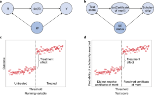
Causation in neuroscience: keeping mechanism meaningful

Causal inference on human behaviour

Comparing meta-analyses and preregistered multiple-laboratory replication projects
Pearl, J. Causality (Cambridge Univ. Press, New York, 2009).
The Notorious B.I.G. Mo’ Money Mo’ Problems (Bad Boy Records, 1997).
Grodstein, F. et al. A prospective, observational study of postmenopausal hormone therapy and primary prevention of cardiovascular disease. Ann. Intern. Med. 133 , 933–941 (2000).
Article CAS Google Scholar
Manson, J. E. et al. Estrogen plus progestin and the risk of coronary heart disease. N. Engl. J. Med. 349 , 523–534 (2003).
Humphrey, L. L., Chan, B. K. & Sox, H. C. Postmenopausal hormone replacement therapy and the primary prevention of cardiovascular disease. Ann. Intern. Med. 137 , 273–284 (2002).
Greenland, S. Randomization, statistics, and causal inference. Epidemiology 1 , 421–429 (1990).
Ismail-Beigi, F. et al. Effect of intensive treatment of hyperglycaemia on microvascular outcomes in type 2 diabetes: an analysis of the ACCORD randomised trial. Lancet 376 , 419–430 (2010).
Article Google Scholar
Officers, T. A. Major outcomes in high-risk hypertensive patients randomized to or calcium channel blocker vs diuretic. J. Am. Med. Assoc. 288 , 2981–2997 (2002).
Group, S. R. A randomized trial of intensive versus standard blood-pressure control. N. Engl. J. Med. 373 , 2103–2116 (2015).
Granger, C. W. Investigating causal relations by econometric models and cross-spectral methods. Econometrica 37 , 424–438 (1969).
Angrist, J. D. & Pischke, J.-S. Mostly Harmless Econometrics: An Empiricist’s Companion (Princeton Univ. Press, Princeton, 2008).
Leamer, E. E. Let’s take the con out of econometrics. Am. Econ. Rev. 73 , 31–43 (1983).
Google Scholar
Thistlethwaite, D. L. & Campbell, D. T. Regression-discontinuity analysis: an alternative to the ex-post facto experiment. J. Educ. Psychol. 51 , 309–317 (1960).
Imbens, G. W. & Lemieux, T. Regression discontinuity designs: a guide to practice. J. Econom. 142 , 615–635 (2008).
Angrist, J., Azoulay, P., Ellison, G., Hill, R. & Lu, S. F. Economic research evolves: fields and styles. Am. Econ. Rev. 107 , 293–297 (2017).
Angrist, J., Azoulay, P., Ellison, G., Hill, R. & Lu, S. F. Inside Job or Deep Impact? Using Extramural Citations to Assess Economic Scholarship (National Bureau of Economic Research, 2017).
McCrary, J. Manipulation of the running variable in the regression discontinuity design: a density test. J. Econom. 142 , 698–714 (2008).
Trochim, W. M. Research Design for Program Evaluation: The Regression-Discontinuity Approach (Sage Publications, Beverly Hills, 1984).
Jacob, R., Zhu, P., Somers, M. A., & Bloom, H. A practical guide to regression discontinuity. MDRC https://www.mdrc.org/publication/practical-guide-regression-discontinuity (2012).
Lansdell, B. & Kording, K. Spiking allows neurons to estimate their causal effect. Preprint at bioRxiv https://doi.org/10.1101/253351 (2018).
Moscoe, E., Bor, J. & Bärnighausen, T. Regression discontinuity designs are underutilized in medicine, epidemiology, and public health: a review of current and best practice. J. Clin. Epidemiol. 68 , 122–133 (2015).
Pischke, J. S. The impact of length of the school year on student performance and earnings: evidence from the German short school years. Econ. J. 117 , 1216–1242 (2007).
Athey, S. & Imbens, G. W. Identification and inference in nonlinear difference-in-differences models. Econometrica 74 , 431–497 (2006).
Angrist, J. D. et al. Identification of causal effects using instrumental variables. J. Am. Stat. Assoc. 91 , 444–455 (2016).
Evans, W. N. & Ringel, J. S. Can higher cigarette taxes improve birth outcomes? J. Public. Econ. 72 , 135–154 (1999).
Stock, J. H. & Yogo, M. Testing for Weak Instruments in Linear IV Regression . (National Bureau of Economic Research, Cambridge, 2002).
Book Google Scholar
Li, X., Yamawaki, N., Barrett, J. M., Körding, K. P. & Shepherd, G. Scaling of optogenetically evoked signaling in a higher-order corticocortical pathway in the anesthetized mouse. Front. Syst. Neurosci . 12 , 16 (2018).
Koller, D. & Friedman, N. Probabilistic Graphical Models: Principles and Techniques (MIT Press, Cambridge, 2009).
Ullman, J. B., & Bentler, P. M. in Handbook of Psychology 2nd edn (eds Schinka, J. A. & Velicer, W. F.) Ch. 23 (John Wiley & Sons, Hoboken, 2012).
Dehejia, R. H. & Wahba, S. Propensity score-matching methods for nonexperimental causal studies. Rev. Econ. Stat. 84 , 151–161 (2002).
Rosenbaum, P. R. & Rubin, D. B. The central role of the propensity score in observational studies for causal effects. Biometrika 70 , 41–55 (1983).
Imbens, G. W. & Rubin, D. B. Causal Inference in Statistics, Social, and Biomedical Sciences (Cambridge Univ. Press, New York, 2015).
Hoyer, P. O., Janzing, D., Mooij, J. M., Peters, J. & Schölkopf, B. Nonlinear causal discovery with additive noise models. Adv. Neural Inf. Process. Syst. 21 , 689–696 (2009).
Abadie, A., Diamond, A. & Hainmueller, J. Synthetic control methods for comparative case studies: estimating the effect of California’s tobacco control program. J. Am. Stat. Assoc. 105 , 493–505 (2010).
Ramsey, J. D. et al. Six problems for causal inference from fMRI. NeuroImage 49 , 1545–1558 (2010).
Jonas, E. & Kording, K. P. Could a neuroscientist understand a microprocessor? PLoS Comput. Biol. 13 , e1005268 (2017).
Valdes-Sosa, P. A., Roebroeck, A., Daunizeau, J. & Friston, K. Effective connectivity: influence, causality and biophysical modeling. NeuroImage 58 , 339–361 (2011).
Smith, S. M., Miller, K. L., Salimi-Khorshidi, G., Webster, M. & Beckmann, C. F. et al. Network modelling methods for FMRI. NeuroImage 54 , 875–891 (2011).
Kwak, H., Lee, C., Park, H. & Moon, S. What is Twitter, a social network or a news media? In Proc. 19th International Conference on World Wide Web 591–600 (ACM, 2010).
Bem, J. Using match confidence to adjust a performance threshold. Google Patent 7346615 (2008).
Slemrod, J. Buenas notches: lines and notches in tax system design. EJ Tax Res. 11 , 259–283 (2013).
Angrist, J. D. & Pischke, J.-S. The credibility revolution in empirical economics: how better research design is taking the con out of econometrics. J. Econ. Perspect. 24 , 3–30 (2010).
Krakauer, J. W., Ghazanfar, A. A., Gomez-Marin, A., MacIver, M. A. & Poeppel, D. Neuroscience needs behavior: correcting a reductionist bias. Neuron (in the press).
Pillow, J. W. et al. Spatio-temporal correlations and visual signalling in a complete neuronal population. Nature 454 , 995–999 (2008).
Stevenson, I. H. & Körding, K. P. On the similarity of functional connectivity between neurons estimated across timescales. PLoS ONE 5 , e9206 (2010).
Sakkalis, V. Review of advanced techniques for the estimation of brain connectivity measured with EEG/MEG. Comput. Biol. Med. 41 , 1110–1117 (2011).
Bressler, S. L. & Seth, A. K. Wiener–Granger causality: a well established methodology. Neuroimage 58 , 323–329 (2011).
Ding, M., Chen, Y. & Bressler, S. L. in Handbook of Time Series Analysis: Recent Theoretical Developments and Applications (eds Schelter, B., Winterhalder, M. & Timmer, J.) 335–368 (Wiley-VCH, Weinheim, 2006).
Hiemstra, C. & Jones, J. D. Testing for linear and nonlinear Granger causality in the stock price — volume relation. J. Finance 49 , 1639–1664 (1994).
Chen, Z. Advanced State Space Methods for Neural and Clinical Data (Cambridge Univ. Press, Cambridge, 2015).
Shumway, R. H. & Stoffer, D. S. in Time Series Analysis and its Applications (Shumway, R. H. & Stoffer, D. S.) 319–404 (Springer, New York, 2011).
Friston, K. J., Harrison, L. & Penny, W. Dynamic causal modelling. NeuroImage 19 , 1273–1302 (2003).
Semedo, J., Zandvakili, A., Kohn, A., Machens, C. K. & Byron, M. Y. Extracting latent structure from multiple interacting neural populations. Adv. Neural Inf. Process. Syst. 27 , 2942–2950 (2014).
Daunizeau, J., David, O. & Stephan, K. E. Dynamic causal modelling: a critical review of the biophysical and statistical foundations. NeuroImage 58 , 312–322 (2009).
Latimer, K. W., Yates, J. L., Meister, M. L. R., Huk, A. C. & Pillow, J. W. Single-trial spike trains in parietal cortex reveal discrete steps during decision-making. Science 349 , 184–187 (2015).
Nevo, A. & Whinston, M. D. Taking the dogma out of econometrics: structural modeling and credible inference. J. Econ. Perspect. 24 , 69–82 (2010).
Song, L., Kolar, M. & Xing, E. P. Time-varying dynamic bayesian networks. Adv. Neural Inf. Process. Syst. 22 , 1732–1740 (2009).
Goodman, N. D., Ullman, T. D. & Tenenbaum, J. B. Learning a theory of causality. Psychol. Rev. 118 , 110–119 (2011).
Gopnik, A. et al. A Theory of causal learning in children: causal maps and Bayes nets. Psychol. Rev. 111 , 3–32 (2004).
Gopnik, A. & Tenenbaum, J. B. Bayesian networks, Bayesian learning and cognitive development. Dev. Sci. 10 , 281–287 (2007).
Körding, K. P. et al. Causal inference in multisensory perception. PLoS ONE 2 , e943 (2007).
Download references
Author information
Authors and affiliations.
Department of Social Policy and Practice, University of Pennsylvania, Philadelphia, PA, USA
Ioana E. Marinescu
Division of Neurology, Children’s Hospital of Philadelphia, Philadelphia, PA, USA
Patrick N. Lawlor
Departments of Neuroscience and Bioengineering, Leonard Davis Institute, Warren Center for Network Science, Wharton Neuroscience Initiative, University of Pennsylvania, Philadelphia, PA, USA
Konrad P. Kording
Canadian Institute For Advanced Research, Toronto, Ontario, Canada
You can also search for this author in PubMed Google Scholar
Corresponding author
Correspondence to Ioana E. Marinescu .
Ethics declarations
Competing interests.
The authors declare no competing interests.
Additional information
Publisher’s note: Springer Nature remains neutral with regard to jurisdictional claims in published maps and institutional affiliations.
Rights and permissions
Reprints and permissions
About this article
Cite this article.
Marinescu, I.E., Lawlor, P.N. & Kording, K.P. Quasi-experimental causality in neuroscience and behavioural research. Nat Hum Behav 2 , 891–898 (2018). https://doi.org/10.1038/s41562-018-0466-5
Download citation
Received : 18 March 2018
Accepted : 02 October 2018
Published : 26 November 2018
Issue Date : December 2018
DOI : https://doi.org/10.1038/s41562-018-0466-5
Share this article
Anyone you share the following link with will be able to read this content:
Sorry, a shareable link is not currently available for this article.
Provided by the Springer Nature SharedIt content-sharing initiative
This article is cited by
- Lauren N. Ross
- Dani S. Bassett
Nature Reviews Neuroscience (2024)
Psychiatric neuroimaging designs for individualised, cohort, and population studies
- Martin Gell
- Stephanie Noble
- Brenden Tervo-Clemmens
Neuropsychopharmacology (2024)
- Drew H. Bailey
- Alexander J. Jung
- Kou Murayama
Nature Human Behaviour (2024)
Workers’ whole day workload and next day cognitive performance
- Raymond Hernandez
- Haomiao Jin
- Stefan Schneider
Current Psychology (2024)
What if we intervene?: Higher-order cross-lagged causal model with interventional approach under observational design
- Christopher Castro
- Kevin Michell
- Marcel C. Minutolo
Neural Computing and Applications (2024)
Quick links
- Explore articles by subject
- Guide to authors
- Editorial policies
Sign up for the Nature Briefing newsletter — what matters in science, free to your inbox daily.

- Privacy Policy
Home » Quasi-Experimental Research Design – Types, Methods
Quasi-Experimental Research Design – Types, Methods
Table of Contents

Quasi-Experimental Design
Quasi-experimental design is a research method that seeks to evaluate the causal relationships between variables, but without the full control over the independent variable(s) that is available in a true experimental design.
In a quasi-experimental design, the researcher uses an existing group of participants that is not randomly assigned to the experimental and control groups. Instead, the groups are selected based on pre-existing characteristics or conditions, such as age, gender, or the presence of a certain medical condition.
Types of Quasi-Experimental Design
There are several types of quasi-experimental designs that researchers use to study causal relationships between variables. Here are some of the most common types:
Non-Equivalent Control Group Design
This design involves selecting two groups of participants that are similar in every way except for the independent variable(s) that the researcher is testing. One group receives the treatment or intervention being studied, while the other group does not. The two groups are then compared to see if there are any significant differences in the outcomes.
Interrupted Time-Series Design
This design involves collecting data on the dependent variable(s) over a period of time, both before and after an intervention or event. The researcher can then determine whether there was a significant change in the dependent variable(s) following the intervention or event.
Pretest-Posttest Design
This design involves measuring the dependent variable(s) before and after an intervention or event, but without a control group. This design can be useful for determining whether the intervention or event had an effect, but it does not allow for control over other factors that may have influenced the outcomes.
Regression Discontinuity Design
This design involves selecting participants based on a specific cutoff point on a continuous variable, such as a test score. Participants on either side of the cutoff point are then compared to determine whether the intervention or event had an effect.
Natural Experiments
This design involves studying the effects of an intervention or event that occurs naturally, without the researcher’s intervention. For example, a researcher might study the effects of a new law or policy that affects certain groups of people. This design is useful when true experiments are not feasible or ethical.
Data Analysis Methods
Here are some data analysis methods that are commonly used in quasi-experimental designs:
Descriptive Statistics
This method involves summarizing the data collected during a study using measures such as mean, median, mode, range, and standard deviation. Descriptive statistics can help researchers identify trends or patterns in the data, and can also be useful for identifying outliers or anomalies.
Inferential Statistics
This method involves using statistical tests to determine whether the results of a study are statistically significant. Inferential statistics can help researchers make generalizations about a population based on the sample data collected during the study. Common statistical tests used in quasi-experimental designs include t-tests, ANOVA, and regression analysis.
Propensity Score Matching
This method is used to reduce bias in quasi-experimental designs by matching participants in the intervention group with participants in the control group who have similar characteristics. This can help to reduce the impact of confounding variables that may affect the study’s results.
Difference-in-differences Analysis
This method is used to compare the difference in outcomes between two groups over time. Researchers can use this method to determine whether a particular intervention has had an impact on the target population over time.
Interrupted Time Series Analysis
This method is used to examine the impact of an intervention or treatment over time by comparing data collected before and after the intervention or treatment. This method can help researchers determine whether an intervention had a significant impact on the target population.
Regression Discontinuity Analysis
This method is used to compare the outcomes of participants who fall on either side of a predetermined cutoff point. This method can help researchers determine whether an intervention had a significant impact on the target population.
Steps in Quasi-Experimental Design
Here are the general steps involved in conducting a quasi-experimental design:
- Identify the research question: Determine the research question and the variables that will be investigated.
- Choose the design: Choose the appropriate quasi-experimental design to address the research question. Examples include the pretest-posttest design, non-equivalent control group design, regression discontinuity design, and interrupted time series design.
- Select the participants: Select the participants who will be included in the study. Participants should be selected based on specific criteria relevant to the research question.
- Measure the variables: Measure the variables that are relevant to the research question. This may involve using surveys, questionnaires, tests, or other measures.
- Implement the intervention or treatment: Implement the intervention or treatment to the participants in the intervention group. This may involve training, education, counseling, or other interventions.
- Collect data: Collect data on the dependent variable(s) before and after the intervention. Data collection may also include collecting data on other variables that may impact the dependent variable(s).
- Analyze the data: Analyze the data collected to determine whether the intervention had a significant impact on the dependent variable(s).
- Draw conclusions: Draw conclusions about the relationship between the independent and dependent variables. If the results suggest a causal relationship, then appropriate recommendations may be made based on the findings.
Quasi-Experimental Design Examples
Here are some examples of real-time quasi-experimental designs:
- Evaluating the impact of a new teaching method: In this study, a group of students are taught using a new teaching method, while another group is taught using the traditional method. The test scores of both groups are compared before and after the intervention to determine whether the new teaching method had a significant impact on student performance.
- Assessing the effectiveness of a public health campaign: In this study, a public health campaign is launched to promote healthy eating habits among a targeted population. The behavior of the population is compared before and after the campaign to determine whether the intervention had a significant impact on the target behavior.
- Examining the impact of a new medication: In this study, a group of patients is given a new medication, while another group is given a placebo. The outcomes of both groups are compared to determine whether the new medication had a significant impact on the targeted health condition.
- Evaluating the effectiveness of a job training program : In this study, a group of unemployed individuals is enrolled in a job training program, while another group is not enrolled in any program. The employment rates of both groups are compared before and after the intervention to determine whether the training program had a significant impact on the employment rates of the participants.
- Assessing the impact of a new policy : In this study, a new policy is implemented in a particular area, while another area does not have the new policy. The outcomes of both areas are compared before and after the intervention to determine whether the new policy had a significant impact on the targeted behavior or outcome.
Applications of Quasi-Experimental Design
Here are some applications of quasi-experimental design:
- Educational research: Quasi-experimental designs are used to evaluate the effectiveness of educational interventions, such as new teaching methods, technology-based learning, or educational policies.
- Health research: Quasi-experimental designs are used to evaluate the effectiveness of health interventions, such as new medications, public health campaigns, or health policies.
- Social science research: Quasi-experimental designs are used to investigate the impact of social interventions, such as job training programs, welfare policies, or criminal justice programs.
- Business research: Quasi-experimental designs are used to evaluate the impact of business interventions, such as marketing campaigns, new products, or pricing strategies.
- Environmental research: Quasi-experimental designs are used to evaluate the impact of environmental interventions, such as conservation programs, pollution control policies, or renewable energy initiatives.
When to use Quasi-Experimental Design
Here are some situations where quasi-experimental designs may be appropriate:
- When the research question involves investigating the effectiveness of an intervention, policy, or program : In situations where it is not feasible or ethical to randomly assign participants to intervention and control groups, quasi-experimental designs can be used to evaluate the impact of the intervention on the targeted outcome.
- When the sample size is small: In situations where the sample size is small, it may be difficult to randomly assign participants to intervention and control groups. Quasi-experimental designs can be used to investigate the impact of an intervention without requiring a large sample size.
- When the research question involves investigating a naturally occurring event : In some situations, researchers may be interested in investigating the impact of a naturally occurring event, such as a natural disaster or a major policy change. Quasi-experimental designs can be used to evaluate the impact of the event on the targeted outcome.
- When the research question involves investigating a long-term intervention: In situations where the intervention or program is long-term, it may be difficult to randomly assign participants to intervention and control groups for the entire duration of the intervention. Quasi-experimental designs can be used to evaluate the impact of the intervention over time.
- When the research question involves investigating the impact of a variable that cannot be manipulated : In some situations, it may not be possible or ethical to manipulate a variable of interest. Quasi-experimental designs can be used to investigate the relationship between the variable and the targeted outcome.
Purpose of Quasi-Experimental Design
The purpose of quasi-experimental design is to investigate the causal relationship between two or more variables when it is not feasible or ethical to conduct a randomized controlled trial (RCT). Quasi-experimental designs attempt to emulate the randomized control trial by mimicking the control group and the intervention group as much as possible.
The key purpose of quasi-experimental design is to evaluate the impact of an intervention, policy, or program on a targeted outcome while controlling for potential confounding factors that may affect the outcome. Quasi-experimental designs aim to answer questions such as: Did the intervention cause the change in the outcome? Would the outcome have changed without the intervention? And was the intervention effective in achieving its intended goals?
Quasi-experimental designs are useful in situations where randomized controlled trials are not feasible or ethical. They provide researchers with an alternative method to evaluate the effectiveness of interventions, policies, and programs in real-life settings. Quasi-experimental designs can also help inform policy and practice by providing valuable insights into the causal relationships between variables.
Overall, the purpose of quasi-experimental design is to provide a rigorous method for evaluating the impact of interventions, policies, and programs while controlling for potential confounding factors that may affect the outcome.
Advantages of Quasi-Experimental Design
Quasi-experimental designs have several advantages over other research designs, such as:
- Greater external validity : Quasi-experimental designs are more likely to have greater external validity than laboratory experiments because they are conducted in naturalistic settings. This means that the results are more likely to generalize to real-world situations.
- Ethical considerations: Quasi-experimental designs often involve naturally occurring events, such as natural disasters or policy changes. This means that researchers do not need to manipulate variables, which can raise ethical concerns.
- More practical: Quasi-experimental designs are often more practical than experimental designs because they are less expensive and easier to conduct. They can also be used to evaluate programs or policies that have already been implemented, which can save time and resources.
- No random assignment: Quasi-experimental designs do not require random assignment, which can be difficult or impossible in some cases, such as when studying the effects of a natural disaster. This means that researchers can still make causal inferences, although they must use statistical techniques to control for potential confounding variables.
- Greater generalizability : Quasi-experimental designs are often more generalizable than experimental designs because they include a wider range of participants and conditions. This can make the results more applicable to different populations and settings.
Limitations of Quasi-Experimental Design
There are several limitations associated with quasi-experimental designs, which include:
- Lack of Randomization: Quasi-experimental designs do not involve randomization of participants into groups, which means that the groups being studied may differ in important ways that could affect the outcome of the study. This can lead to problems with internal validity and limit the ability to make causal inferences.
- Selection Bias: Quasi-experimental designs may suffer from selection bias because participants are not randomly assigned to groups. Participants may self-select into groups or be assigned based on pre-existing characteristics, which may introduce bias into the study.
- History and Maturation: Quasi-experimental designs are susceptible to history and maturation effects, where the passage of time or other events may influence the outcome of the study.
- Lack of Control: Quasi-experimental designs may lack control over extraneous variables that could influence the outcome of the study. This can limit the ability to draw causal inferences from the study.
- Limited Generalizability: Quasi-experimental designs may have limited generalizability because the results may only apply to the specific population and context being studied.
About the author

Muhammad Hassan
Researcher, Academic Writer, Web developer
You may also like

Descriptive Research Design – Types, Methods and...

Basic Research – Types, Methods and Examples

Triangulation in Research – Types, Methods and...

Case Study – Methods, Examples and Guide

Textual Analysis – Types, Examples and Guide

Focus Groups – Steps, Examples and Guide
Want to create or adapt books like this? Learn more about how Pressbooks supports open publishing practices.
Chapter 7: Nonexperimental Research
Quasi-Experimental Research
Learning Objectives
- Explain what quasi-experimental research is and distinguish it clearly from both experimental and correlational research.
- Describe three different types of quasi-experimental research designs (nonequivalent groups, pretest-posttest, and interrupted time series) and identify examples of each one.
The prefix quasi means “resembling.” Thus quasi-experimental research is research that resembles experimental research but is not true experimental research. Although the independent variable is manipulated, participants are not randomly assigned to conditions or orders of conditions (Cook & Campbell, 1979). [1] Because the independent variable is manipulated before the dependent variable is measured, quasi-experimental research eliminates the directionality problem. But because participants are not randomly assigned—making it likely that there are other differences between conditions—quasi-experimental research does not eliminate the problem of confounding variables. In terms of internal validity, therefore, quasi-experiments are generally somewhere between correlational studies and true experiments.
Quasi-experiments are most likely to be conducted in field settings in which random assignment is difficult or impossible. They are often conducted to evaluate the effectiveness of a treatment—perhaps a type of psychotherapy or an educational intervention. There are many different kinds of quasi-experiments, but we will discuss just a few of the most common ones here.
Nonequivalent Groups Design
Recall that when participants in a between-subjects experiment are randomly assigned to conditions, the resulting groups are likely to be quite similar. In fact, researchers consider them to be equivalent. When participants are not randomly assigned to conditions, however, the resulting groups are likely to be dissimilar in some ways. For this reason, researchers consider them to be nonequivalent. A nonequivalent groups design , then, is a between-subjects design in which participants have not been randomly assigned to conditions.
Imagine, for example, a researcher who wants to evaluate a new method of teaching fractions to third graders. One way would be to conduct a study with a treatment group consisting of one class of third-grade students and a control group consisting of another class of third-grade students. This design would be a nonequivalent groups design because the students are not randomly assigned to classes by the researcher, which means there could be important differences between them. For example, the parents of higher achieving or more motivated students might have been more likely to request that their children be assigned to Ms. Williams’s class. Or the principal might have assigned the “troublemakers” to Mr. Jones’s class because he is a stronger disciplinarian. Of course, the teachers’ styles, and even the classroom environments, might be very different and might cause different levels of achievement or motivation among the students. If at the end of the study there was a difference in the two classes’ knowledge of fractions, it might have been caused by the difference between the teaching methods—but it might have been caused by any of these confounding variables.
Of course, researchers using a nonequivalent groups design can take steps to ensure that their groups are as similar as possible. In the present example, the researcher could try to select two classes at the same school, where the students in the two classes have similar scores on a standardized math test and the teachers are the same sex, are close in age, and have similar teaching styles. Taking such steps would increase the internal validity of the study because it would eliminate some of the most important confounding variables. But without true random assignment of the students to conditions, there remains the possibility of other important confounding variables that the researcher was not able to control.
Pretest-Posttest Design
In a pretest-posttest design , the dependent variable is measured once before the treatment is implemented and once after it is implemented. Imagine, for example, a researcher who is interested in the effectiveness of an antidrug education program on elementary school students’ attitudes toward illegal drugs. The researcher could measure the attitudes of students at a particular elementary school during one week, implement the antidrug program during the next week, and finally, measure their attitudes again the following week. The pretest-posttest design is much like a within-subjects experiment in which each participant is tested first under the control condition and then under the treatment condition. It is unlike a within-subjects experiment, however, in that the order of conditions is not counterbalanced because it typically is not possible for a participant to be tested in the treatment condition first and then in an “untreated” control condition.
If the average posttest score is better than the average pretest score, then it makes sense to conclude that the treatment might be responsible for the improvement. Unfortunately, one often cannot conclude this with a high degree of certainty because there may be other explanations for why the posttest scores are better. One category of alternative explanations goes under the name of history . Other things might have happened between the pretest and the posttest. Perhaps an antidrug program aired on television and many of the students watched it, or perhaps a celebrity died of a drug overdose and many of the students heard about it. Another category of alternative explanations goes under the name of maturation . Participants might have changed between the pretest and the posttest in ways that they were going to anyway because they are growing and learning. If it were a yearlong program, participants might become less impulsive or better reasoners and this might be responsible for the change.
Another alternative explanation for a change in the dependent variable in a pretest-posttest design is regression to the mean . This refers to the statistical fact that an individual who scores extremely on a variable on one occasion will tend to score less extremely on the next occasion. For example, a bowler with a long-term average of 150 who suddenly bowls a 220 will almost certainly score lower in the next game. Her score will “regress” toward her mean score of 150. Regression to the mean can be a problem when participants are selected for further study because of their extreme scores. Imagine, for example, that only students who scored especially low on a test of fractions are given a special training program and then retested. Regression to the mean all but guarantees that their scores will be higher even if the training program has no effect. A closely related concept—and an extremely important one in psychological research—is spontaneous remission . This is the tendency for many medical and psychological problems to improve over time without any form of treatment. The common cold is a good example. If one were to measure symptom severity in 100 common cold sufferers today, give them a bowl of chicken soup every day, and then measure their symptom severity again in a week, they would probably be much improved. This does not mean that the chicken soup was responsible for the improvement, however, because they would have been much improved without any treatment at all. The same is true of many psychological problems. A group of severely depressed people today is likely to be less depressed on average in 6 months. In reviewing the results of several studies of treatments for depression, researchers Michael Posternak and Ivan Miller found that participants in waitlist control conditions improved an average of 10 to 15% before they received any treatment at all (Posternak & Miller, 2001) [2] . Thus one must generally be very cautious about inferring causality from pretest-posttest designs.
Does Psychotherapy Work?
Early studies on the effectiveness of psychotherapy tended to use pretest-posttest designs. In a classic 1952 article, researcher Hans Eysenck summarized the results of 24 such studies showing that about two thirds of patients improved between the pretest and the posttest (Eysenck, 1952) [3] . But Eysenck also compared these results with archival data from state hospital and insurance company records showing that similar patients recovered at about the same rate without receiving psychotherapy. This parallel suggested to Eysenck that the improvement that patients showed in the pretest-posttest studies might be no more than spontaneous remission. Note that Eysenck did not conclude that psychotherapy was ineffective. He merely concluded that there was no evidence that it was, and he wrote of “the necessity of properly planned and executed experimental studies into this important field” (p. 323). You can read the entire article here: Classics in the History of Psychology .
Fortunately, many other researchers took up Eysenck’s challenge, and by 1980 hundreds of experiments had been conducted in which participants were randomly assigned to treatment and control conditions, and the results were summarized in a classic book by Mary Lee Smith, Gene Glass, and Thomas Miller (Smith, Glass, & Miller, 1980) [4] . They found that overall psychotherapy was quite effective, with about 80% of treatment participants improving more than the average control participant. Subsequent research has focused more on the conditions under which different types of psychotherapy are more or less effective.
Interrupted Time Series Design
A variant of the pretest-posttest design is the interrupted time-series design . A time series is a set of measurements taken at intervals over a period of time. For example, a manufacturing company might measure its workers’ productivity each week for a year. In an interrupted time series-design, a time series like this one is “interrupted” by a treatment. In one classic example, the treatment was the reduction of the work shifts in a factory from 10 hours to 8 hours (Cook & Campbell, 1979) [5] . Because productivity increased rather quickly after the shortening of the work shifts, and because it remained elevated for many months afterward, the researcher concluded that the shortening of the shifts caused the increase in productivity. Notice that the interrupted time-series design is like a pretest-posttest design in that it includes measurements of the dependent variable both before and after the treatment. It is unlike the pretest-posttest design, however, in that it includes multiple pretest and posttest measurements.
Figure 7.3 shows data from a hypothetical interrupted time-series study. The dependent variable is the number of student absences per week in a research methods course. The treatment is that the instructor begins publicly taking attendance each day so that students know that the instructor is aware of who is present and who is absent. The top panel of Figure 7.3 shows how the data might look if this treatment worked. There is a consistently high number of absences before the treatment, and there is an immediate and sustained drop in absences after the treatment. The bottom panel of Figure 7.3 shows how the data might look if this treatment did not work. On average, the number of absences after the treatment is about the same as the number before. This figure also illustrates an advantage of the interrupted time-series design over a simpler pretest-posttest design. If there had been only one measurement of absences before the treatment at Week 7 and one afterward at Week 8, then it would have looked as though the treatment were responsible for the reduction. The multiple measurements both before and after the treatment suggest that the reduction between Weeks 7 and 8 is nothing more than normal week-to-week variation.

Combination Designs
A type of quasi-experimental design that is generally better than either the nonequivalent groups design or the pretest-posttest design is one that combines elements of both. There is a treatment group that is given a pretest, receives a treatment, and then is given a posttest. But at the same time there is a control group that is given a pretest, does not receive the treatment, and then is given a posttest. The question, then, is not simply whether participants who receive the treatment improve but whether they improve more than participants who do not receive the treatment.
Imagine, for example, that students in one school are given a pretest on their attitudes toward drugs, then are exposed to an antidrug program, and finally are given a posttest. Students in a similar school are given the pretest, not exposed to an antidrug program, and finally are given a posttest. Again, if students in the treatment condition become more negative toward drugs, this change in attitude could be an effect of the treatment, but it could also be a matter of history or maturation. If it really is an effect of the treatment, then students in the treatment condition should become more negative than students in the control condition. But if it is a matter of history (e.g., news of a celebrity drug overdose) or maturation (e.g., improved reasoning), then students in the two conditions would be likely to show similar amounts of change. This type of design does not completely eliminate the possibility of confounding variables, however. Something could occur at one of the schools but not the other (e.g., a student drug overdose), so students at the first school would be affected by it while students at the other school would not.
Finally, if participants in this kind of design are randomly assigned to conditions, it becomes a true experiment rather than a quasi experiment. In fact, it is the kind of experiment that Eysenck called for—and that has now been conducted many times—to demonstrate the effectiveness of psychotherapy.
Key Takeaways
- Quasi-experimental research involves the manipulation of an independent variable without the random assignment of participants to conditions or orders of conditions. Among the important types are nonequivalent groups designs, pretest-posttest, and interrupted time-series designs.
- Quasi-experimental research eliminates the directionality problem because it involves the manipulation of the independent variable. It does not eliminate the problem of confounding variables, however, because it does not involve random assignment to conditions. For these reasons, quasi-experimental research is generally higher in internal validity than correlational studies but lower than true experiments.
- Practice: Imagine that two professors decide to test the effect of giving daily quizzes on student performance in a statistics course. They decide that Professor A will give quizzes but Professor B will not. They will then compare the performance of students in their two sections on a common final exam. List five other variables that might differ between the two sections that could affect the results.
- regression to the mean
- spontaneous remission
Image Descriptions
Figure 7.3 image description: Two line graphs charting the number of absences per week over 14 weeks. The first 7 weeks are without treatment and the last 7 weeks are with treatment. In the first line graph, there are between 4 to 8 absences each week. After the treatment, the absences drop to 0 to 3 each week, which suggests the treatment worked. In the second line graph, there is no noticeable change in the number of absences per week after the treatment, which suggests the treatment did not work. [Return to Figure 7.3]
- Cook, T. D., & Campbell, D. T. (1979). Quasi-experimentation: Design & analysis issues in field settings . Boston, MA: Houghton Mifflin. ↵
- Posternak, M. A., & Miller, I. (2001). Untreated short-term course of major depression: A meta-analysis of studies using outcomes from studies using wait-list control groups. Journal of Affective Disorders, 66 , 139–146. ↵
- Eysenck, H. J. (1952). The effects of psychotherapy: An evaluation. Journal of Consulting Psychology, 16 , 319–324. ↵
- Smith, M. L., Glass, G. V., & Miller, T. I. (1980). The benefits of psychotherapy . Baltimore, MD: Johns Hopkins University Press. ↵
A between-subjects design in which participants have not been randomly assigned to conditions.
The dependent variable is measured once before the treatment is implemented and once after it is implemented.
A category of alternative explanations for differences between scores such as events that happened between the pretest and posttest, unrelated to the study.
An alternative explanation that refers to how the participants might have changed between the pretest and posttest in ways that they were going to anyway because they are growing and learning.
The statistical fact that an individual who scores extremely on a variable on one occasion will tend to score less extremely on the next occasion.
The tendency for many medical and psychological problems to improve over time without any form of treatment.
A set of measurements taken at intervals over a period of time that are interrupted by a treatment.
Research Methods in Psychology - 2nd Canadian Edition Copyright © 2015 by Paul C. Price, Rajiv Jhangiani, & I-Chant A. Chiang is licensed under a Creative Commons Attribution-NonCommercial-ShareAlike 4.0 International License , except where otherwise noted.
Share This Book

An official website of the United States government
The .gov means it’s official. Federal government websites often end in .gov or .mil. Before sharing sensitive information, make sure you’re on a federal government site.
The site is secure. The https:// ensures that you are connecting to the official website and that any information you provide is encrypted and transmitted securely.
- Publications
- Account settings
Preview improvements coming to the PMC website in October 2024. Learn More or Try it out now .
- Advanced Search
- Journal List
- HHS Author Manuscripts
Selecting and Improving Quasi-Experimental Designs in Effectiveness and Implementation Research
Margaret a. handley.
1 Department of Epidemiology and Biostatistics, Division of Infectious Disease Epidemiology, University of California, San Francisco, CA
2 General Internal Medicine and UCSF Center for Vulnerable Populations, San Francisco Zuckerberg General Hospital and Trauma Center, University of California, San Francisco, CA, 1001 Potrero Avenue, Box 1364, San Francisco, CA 94110
Courtney Lyles
Charles mcculloch, adithya cattamanchi.
3 Division of Pulmonary and Critical Care Medicine and UCSF Center for Vulnerable Populations, San Francisco Zuckerberg General Hospital and Trauma Center, University of California, San Francisco, CA, 1001 Potrero Avenue, San Francisco, CA 94110
Interventional researchers face many design challenges when assessing intervention implementation in real-world settings. Intervention implementation requires ‘holding fast’ on internal validity needs while incorporating external validity considerations (such as uptake by diverse sub-populations, acceptability, cost, sustainability). Quasi-experimental designs (QEDs) are increasingly employed to achieve a better balance between internal and external validity. Although these designs are often referred to and summarized in terms of logistical benefits versus threats to internal validity, there is still uncertainty about: (1) how to select from among various QEDs, and (2) strategies to strengthen their internal and external validity. We focus on commonly used QEDs (pre-post designs with non-equivalent control groups, interrupted time series, and stepped wedge designs) and discuss several variants that maximize internal and external validity at the design, execution, and analysis stages.
INTRODUCTION
Public health practice involves implementation or adaptation of evidence-based interventions into new settings in order to improve health for individuals and populations. Such interventions typically include on one or more of the “7 Ps” (programs, practices, principles, procedures, products, pills, and policies) ( 9 ). Increasingly, both public health and clinical research have sought to generate practice-based evidence on a wide range of interventions, which in turn has led to a greater focus on intervention research designs that can be applied in real-world settings ( 2 , 8 , 9 , 20 , 25 , 26 , 10 , 2 ).
Randomized controlled trials (RCTs) in which individuals are assigned to intervention or control (standard-of-care or placebo) arms are considered the gold standard for assessing causality and as such are a first choice for most intervention research. Random allocation minimizes selection bias and maximizes the likelihood that measured and unmeasured confounding variables are distributed equally, enabling any difference in outcomes between intervention and control arms to be attributed to the intervention under study. RCTs can also involve random assignment of groups (e.g., clinics, worksites or communities) to intervention and control arms, but a large number of groups are required in order to realize the full benefits of randomization. Traditional RCTs strongly prioritize internal validity over external validity by employing strict eligibility criteria and rigorous data collection methods.
Alternative research methods are needed to test interventions for their effectiveness in many real-world settings—and later when evidence-based interventions are known, for spreading or scaling up these interventions to new settings and populations ( 23 , 40 ). In real-world settings, random allocation of the intervention may not be possible or fully under the control of investigators because of practical, ethical, social, or logistical constraints. For example, when partnering with communities or organizations to deliver a public health intervention, it might not be acceptable that only half of individuals or sites receive an intervention. As well, the timing of intervention roll-out might be determined by an external process outside the control of the investigator, such as a mandated policy. Also, when self-selected groups are expected to participate in a program as part of routine care, there would arise ethical concerns associated with random assignment – for example, the withholding or delaying of a potentially effective treatment or the provision of a less effective treatment for one group of participants ( 49 ). As described by Peters et al “implementation research seeks to understand and work within real world conditions, rather than trying to control for these conditions or to remove their influence as causal effects. “ ( 40 ). For all of these reasons, a blending of the design components of clinical effectiveness trials and implementation research is feasible and desirable, and this review covers both. Such blending of effectiveness and implementation components within a study can provide benefits beyond either research approach alone ( 14 ), for example by leading to faster uptake of interventions by simultaneously testing implementation strategies.
Since assessment of intervention effectiveness and implementation in real-world settings requires increased focus on external validity (including consideration of factors enhancing intervention uptake by diverse sub-populations, acceptability to a wide range of stakeholders, cost, and sustainability) ( 34 ), interventional research designs are needed that are more relevant to the potential, ‘hoped for’ treatment population than a RCT, and that achieve a better balance between internal and external validity. Quasi-experimental designs (QEDs), which first gained prominence in social science research ( 11 ), are increasingly being employed to fill this need. [ BOX 1 HERE: Definitions used in this review].
DEFINITIONS AND TERMS USED IN PAPER
| Terms and Definitions | |
|---|---|
| Quasi-Experimental Design: | QEDs include a wide range of nonrandomized or partially randomized pre-post intervention studies |
| Pre-Post Design | A QED with data collected before and after an intervention is introduced, and then the compared. An added control group can be added for a Pre-Post Design with a Non-Equivalent control group |
| Non-Equivalent Control Group | A control group that is not randomly assigned to receive or not receive the intervention. Usually, an intact group is selected that is thought to be similar to the intervention group. |
| Interrupted Time Series Design | Multiple observations are evaluated for several consecutive points in time before and after intervention within the same individual or group |
| Stepped Wedge Design | A type of crossover design where the time of crossover is randomized |
| Wash out period | Time period for which a prior practice or intervention is stopped, and a new one is implemented, for which both interventions may be operating, and thus the data is excluded. |
| Inverse Roll-Out | Sites are rolled out to receive the intervention using a structured approach to create balance between the sites over the roll-out time period, using a sample characteristic that is ordered (and then reverse ordered). Commonly size or geography may be used. (e.g. 1,2,3,4 for size followed by 4,3,2,1) |
| Partial Randomization | A type of stratified randomization, with strata constructed for potential confounding variables and randomization occurs separately within each stratum (also called blocked randomization) |
| Internal Validity | Internal validity refers to the extent to which a study is capable of establishing causality is related to the degree it minimizes error or bias |
| External Validity | External validity describes the extent to which a research conclusion can be generalized to the population or to other settings |
QEDs test causal hypotheses but, in lieu of fully randomized assignment of the intervention, seek to define a comparison group or time period that reflects the counter-factual ( i.e., outcomes if the intervention had not been implemented) ( 43 ). QEDs seek to identify a comparison group or time period that is as similar as possible to the treatment group or time period in terms of baseline (pre-intervention) characteristics. QEDs can include partial randomization such as in stepped wedge designs (SWD) when there is pre-determined (and non-random) stratification of sites, but the order in which sites within each strata receive the intervention is assigned randomly. For example, strata that are determined by size or perceived ease of implementation may be assigned to receive the intervention first. However, within those strata the specific sites themselves are randomly selected to receive the intervention across the time intervals included in the study). In all cases, the key threat to internal validity of QEDs is a lack of similarity between the comparison and intervention groups or time periods due to differences in characteristics of the people, sites, or time periods involved.
Previous reviews in this journal have focused on the importance and use of QEDs and other methods to enhance causal inference when evaluating the impact of an intervention that has already been implemented ( 4 , 8 , 9 , 18 ). Design approaches in this case often include creating a post-hoc comparison group for a natural experiment or identifying pre and post-intervention data to then conduct an interrupted time series study. Analysis phase approaches often utilize techniques such as pre-post, regression adjustment, scores, difference-in-differences, synthetic controls, interrupted time series, regression discontinuity, and instrumental variables ( 4 , 9 , 18 ). Although these articles summarize key components of QEDs (e.g. interrupted time series), as well as analysis-focused strategies (regression adjustment, propensity scores, difference-in-differences, synthetic controls, and instrumental variables) there is still uncertainty about: (1) how to select from among various QEDs in the pre-implementation design phase, and (2) strategies to strengthen internal and external validity before and during the implementation phase.
In this paper we discuss the a priori choice of a QED when evaluating the impact of an intervention or policy for which the investigator has some element of design control related to 1) order of intervention allocation (including random and non-random approaches); 2) selecting sites or individuals; and/or 3) timing and frequency of data collection. In the next section, we discuss the main QEDs used for prospective evaluations of interventions in real-world settings and their advantages and disadvantages with respect to addressing threats to internal validity [ BOX 2 HERE Common Threats to Internal Validty of Quasi-Experimental Designs Evaluating Interventions in ‘Real World’ Settings]. Following this summary, we discuss opportunities to strengthen their internal validity, illustrated with examples from the literature. Then we propose a decision framework for key decision points that lead to different QED options. We conclude with a brief discussion of incorporating additional design elements to capture the full range of relevant implementation outcomes in order to maximize external validity.
Common Threats to Internal Validty of Quasi-Experimental Designs Evaluating Interventions in ‘Real World’ Settings
| History Bias | Events other than the intervetion occuring at the same time may influence the results |
| Selection Bias | Systematic differences in subject characteristics between intervention and control groups that are related to the outcome |
| Maturation Bias | Occurs when changes occur to individuals in the groups, differently, over time resulting in effects, in addition to (or rather than) the treatment condition, that may change the performance of participants in the post-test relative to the pre-test |
| Lack of Blinding | Awareness of group assignement can influence those delivering or receiving the intervetion |
| Differential Drop-Out | Attrition that may affect either intervention or control groups differently and result in selection bias and/or loss of statistical power |
| Variability in interactive effects | Implementation of intervention with multiple components may vary across the implementation process and by sites |
QUASI-EXPERIMENTAL DESIGNS FOR PROSPECTIVE EVALUTION OF INTERVENTIONS
Table 1 summarizes the main QEDs that have been used for prospective evaluation of health intervention in real-world settings; pre-post designs with a non-equivalent control group, interrupted time series and stepped wedge designs. We do not include pre-post designs without a control group in this review, as in general, QEDs are primarily those designs that identify a comparison group or time period that is as similar as possible to the treatment group or time period in terms of baseline (pre-intervention) characteristics ( 50 ). Below, we describe features of each QED, considering strengths and limitations and providing examples of their use.
Overview of Commonly Used QED in Intervention Research*
| QED Design | Key Design Elements | Advantages | Disadvantages |
|---|---|---|---|
| Pre-Post with Non-equivalent control group | Comparison of those receiving the intervention with those not receiving it. Analysis is usually based on estimating the difference in the amount of change over time in the outcome of interest between the two groups, beginning with the intervention and moving forward in time; The two groups can also be a different group examined using a before and after intervention cohort | Simplicity of data collection, when smaller number of time points, and associated lower cost; less cumbersome to implement than other designs | Temporal biases are a substantial risk and may result in regression to the mean or over-interpretation of intervention effects; quality of data may vary in different time periods resulting in measurement error; non-equivalent sites may not be comparable for important covariates |
| Interrupted Time Series | Multiple observations are assessed for a number of consecutive points in time before and after intervention within the same individual or group | Useful for when there is a small number of communities or groups, as each group acts as their own control May be only option for studying impacts of large scale health policies | Requires a large number of measurements, may not be feasible for geographically dispersed areas |
| Stepped Wedge Design | Intervention is rolled out over time, usually at the site level. Participants who initially do not receive the intervention later-cross over to receive the intervention. Those that wait, provide control data during the time others receive the intervention, reducing the risk of bias due to time and time-dependent covariates. Can either be based on serial cross-sectional data collected by sites for different time periods (sites cross over) or by following a cohort of same individuals over time (individuals cross over) | All clusters or wait list groups eventually receives the intervention; Do not need to supply intervention in all sites in a short time frame “staggered implementation” | May not be able to randomly assign roll-out of sites, thereby potentially jeopardizing internal validity Cannot guarantee everyone in each cluster or list will receive the intervention during the time that cluster is receiving the intervention -Often takes longer than other designs to implement -Control data must be collected or ascertained from sites or participants -Site differences and implementation processes can vary significantly over time -Risk of contamination in later sites or intervention fatigue – both can wash out potential intervention effects |
1. Pre-Post With Non-Equivalent Control Group
The first type of QED highlighted in this review is perhaps the most straightforward type of intervention design: the pre-post comparison study with a non-equivalent control group. In this design, the intervention is introduced at a single point in time to one or more sites, for which there is also a pre-test and post-test evaluation period, The pre-post differences between these two sites is then compared. In practice, interventions using this design are often delivered at a higher level, such as to entire communities or organizations 1 [ Figure 1 here]. In this design the investigators identify additional site(s) that are similar to the intervention site to serve as a comparison/control group. However, these control sites are different in some way than the intervention site(s) and thus the term “non-equivalent” is important, and clarifies that there are inherent differences in the treatment and control groups ( 15 ).

Illustration of the Pre-Post Non-Equivalent Control Group Design
The strengths of pre-post designs are mainly based in their simplicity, such as data collection is usually only at a few points (although sometimes more). However, pre-post designs can be affected by several of the threats to internal validity of QEDs presented here. The largest challenges are related to 1) ‘history bias’ in which events unrelated to the intervention occur (also referred to as secular trends) before or during the intervention period and have an effect on the outcome (either positive or negative) that are not related to the intervention ( 39 ); and 2) differences between the intervention and control sites because the non-equivalent control groups are likely to differ from the intervention sites in a number of meaningful ways that impact the outcome of interest and can bias results (selection bias).
At this design stage, the first step at improving internal validity would be focused on selection of a non-equivalent control group(s) for which some balance in the distribution of known risk factors is established. This can be challenging as there may not be adequate information available to determine how ‘equivalent’ the comparison group is regarding relevant covariates.
It can be useful to obtain pre-test data or baseline characteristics to improve the comparability of the two groups. In the most controlled situations within this design, the investigators might include elements of randomization or matching for individuals in the intervention or comparison site, to attempt to balance the covariate distribution. Implicit in this approach is the assumption that the greater the similarity between groups, the smaller the likelihood that confounding will threaten inferences of causality of effect for the intervention ( 33 , 47 ). Thus, it is important to select this group or multiple groups with as much specificity as possible.
In order to enhance the causal inference for pre-post designs with non-equivalent control groups, the best strategies improve the comparability of the control group with regards to potential covariates related to the outcome of interest but are not under investigation. One strategy involves creating a cohort, and then using targeted sampling to inform matching of individuals within the cohort. Matching can be based on demographic and other important factors (e.g. measures of health care access or time-period). This design in essence creates a matched, nested case-control design.
Collection of additional data once sites are selected cannot in itself reduce bias, but can inform the examination of the association of interest, and provide data supporting interpretation consistent with the reduced likelihood of bias. These data collection strategies include: 1) extra data collection points at additional pre- or post- time points (to get closer to an interrupted time series design in effect and examine potential threats of maturation and history bias), and 2) collection of data on other dependent variables with a priori assessment of how they will ‘react’ with time dependent variables. A detailed analysis can then provide information on the potential affects on the outcome of interest (to understand potential underlying threats due to history bias).
Additionally, there are analytic strategies that can improve the interpretation of this design, such as: 1) analysis for multiple non-equivalent control groups, to determine if the intervention effects are robust across different conditions or settings (.e.g. using sensitivity analysis), 2) examination within a smaller critical window of the study in which the intervention would be plausibly expected to make the most impact, and 3) identification of subgroups of individuals within the intervention community who are known to have received high vs. low exposure to the intervention, to be able to investigate a potential “dose-response” effect. Table 2 provides examples of studies using the pre-post non-equivalent control group designs that have employed one or more of these improvement approaches to improve the internal study’s validity.
Improving Quasi-Experimental Designs-Internal and External Validity Considerations
| Study/General Design | Intervention | Design Strategy to Improve Internal Validity | Design Strategy to Improve External Validity |
| Pre-Post Designs with Non-Equivalent Control Group | |||
| Cousins et al 2016 | Campus Watch program targeting problem drinking and violence at 1 university campus with 5 control campuses in New Zealand | • Standardization of independent repeat sampling, survey and follow-up methods across all sites (5 control and 1 intervention site) • 5 sites as controls studies aggregate and individually as controls • Consumption and harms data from national surveys to compare data trends over time | Over-sampling of indigenous groups to extend interpretation of findings |
| Chronic disease management program with pharmacist-based patient coaching within a health care insurance plan in Cincinnati, US | • Matching of participants with non-participants on demographic and health care access measures (using propensity score matching) | ||
| Distribution of bed nets to prevent malaria and reduce malaria mortality in Gambia 41 sites receiving intervention compared to external villages (which differed by size and ethnic distribution) | • Examination of data trends during the highest infection times of the year (i.e., rainy season vs dry season) to see if rates were higher then. • Detailed study of those using bed nets within intervention villages (i.e., guaranteed exposure “dose”, to examine dose-response in intervention arm | ||
| Interrupted Time Series | |||
| Study/General Design | Intervention | Design Strategy to Improve Internal Validity | Design Strategy to Improve External Validity |
| Pellegrin 2016 Interrupted time series with comparison group | Formal transfer of high-risk patients being discharged from hospital to a community-based pharmacist follow-up program for up to 1 year post-hospitalization (6 intervention and 5 control sites) | • Long baseline period (12 pre-intervention data points) • Intervention roll-out staggered based on staff availability (site 1 had eight post-intervention data points while site 8 had two) | Detailed implementation-related process measures monitored (and provided to individual community-based pharmacists regarding their performance) over entire study period |
| Robinson 2015 Interrupted time series without control group | New hospital discharge program to support high-risk patients with nurse telephone follow-up and referral to specific services (such as pharmacists for medication reconciliation and review) | • Additionally examined regression discontinuity during the intervention period to determine if the risk score used to determine eligibility for the program influenced the outcome | Measured implementation outcomes of whether the intervention was delivered with high fidelity to the protocols |
| Interrupted time series with comparison group | Removal of direct payment at point of health care services for children under 5, very low income individuals and pregnant women re: consultations, medications and hospitalizations | Built into a pilot to collect control data, and then extend this work to include additional districts, one intervention and one non-intervention district, along with 6 additional years of observation. | Examined sustainability over 72 months of follow-up, and associations with clinic characteristics, such as density of workforce. |
| Stepped Wedge Design | |||
| Study/General Design | Intervention | Design Strategy to Improve Internal Validity | Design Strategy to Improve External Validity |
| Non-randomized stepped wedge cluster trial | Site-level roll out of integrated antiretroviral treatment (ART) intervention in 8 public sector clinics, to achieve more rapid treatment initiation among women with HIV in Zambia, than the existing referral method used for initiation of treatment. | • The 8 sites were matched into four pairs based on the number of HIV-infected pregnant women expected in each site. • The intervention roll out was done for one member of the least busy pair, one member of the second busiest pair, one member of the third busiest pair, and one member of the busiest pair. Rollout to the remaining pairs proceeded in reverse order. • A transition cohort was established that was later excluded from the analysis. It included women who were identified as eligible in the control period of time close to the time the intervention was starting. | |
| See also: Randomized stepped wedge cluster trial | Multi-faceted quality improvement intervention with a passive and an active phase among 6 regional emergency medical services systems and 32 academic and community hospitals in Ontario, Canada. The intervention focused on comparing interventions to improve the implementation of targeted temperature management following out-of-hospital cardiac arrest through passive (education, generic protocol, order set, local champions) versus additional active quality improvement interventions (nurse specialist providing site-specific interven- tions, monthly audit-feedback, network educational events, inter- net blog) versus no intervention (baseline standard of care). | : • Randomization at the level of the hospital, rather than the patient to minimize contamination, since the intervention targeted groups of clinicians. • Hospitals were stratified by number of Intensive Care Unit beds ((< 10 beds vs ≥ 10 beds as a proxy for hospital size). Randomization was done within strata. • Formalized a transition cohort for which a more passive intervention strategy was tested. This also allowed more time for sites to adopt all elements of the complex intervention before crossing over to the active intervention group. | Characterization of system and organizational factors that might affect adoption: Collection of longitudinal data relevant to implementation processes that could impact interpretation of findings such as academic vs community affiliation, urban vs rural (bed size) |
| Randomized stepped wedge cluster trial | Seasonal malaria prophylaxis for children up to age 10 in central Senegal given to households monthly through health system staff led home visits during the malaria season. The first two phases of implementation focused on children under age 5 years and the last phase included children up to age 10 years, and maintained a control only group of sites during this period. | : • Constrained randomization of program roll-out across 54 health posts catchment areas and center-covered regions, • More sites received the intervention later stages (n=18) than in beginning (n=9). • To achieve balance within settings for potential confounders (since they did not have data on malaria incidence), such as distance from river, distance from health center, population size and number of villages, assessment of ability to implement. • Included nine clinics as control sites throughout the study period. | Characterization of factors that might affect usage and adherence made with longitudinal data: Independent evaluations of malaria prophylaxis usage, adherence, and acceptance were included prospectively, using routine health cards at family level and with external assessments from community surveys. In-depth interviews conducted across community levels to understand acceptability and other responses to the intervention Included an embedded study broadening inclusion criteria, to focus on a wider age group of at risk children |
| Wait-list randomized stepped wedge design | Enrollment of 1,655 male mine employees with HIV infection randomized over a short period of time into an intervention to prevent TB infection (use of isoniazid preventive therapy), among individuals with HIV. Treatment was self-administered for 6 months or for 12 months and results were based on cohort analyses. | • Employees were invited in random sequence to attend a workplace HIV clinic. | Enumeration of at risk cohort and estimation of spill-over effect beyond those enrolled: Since they used an enrollment list, they were able to estimate the effect of the intervention (the provision of clinic services) among the entire eligible population, not just those enrolled in the intervention over the study period. |
| Ratanawongsa et al; Handley et al 2011 Wait-list randomized stepped wedge design | Enrollment of 362 patients with diabetes into a health-IT enabled self-management support telephone coaching program, using a wait-list generated from a regional health plan, delivered in 3 languages. | • Patients were identified from an actively maintained diabetes registry covering 4 safety net health clinics in the United States, and randomized to receive the coaching intervention immediately or after 6 moths. • Patients were randomized to balance enrolment for English, Cantonese, and Spanish, over the study period. | External validity-related measures for acceptability among patients as well as fidelity measures, for the health IT-enabled health coaching intervention were assessed using a fidelity framework. |
| Bailet et al 2011 | Literacy intervention for pre-kindergarten children at risk for reading failure in a southern US city administered in child care and pre-school sites, delivered twice a week for 9 weeks. For large sites, did not randomize at site level, but split the schools, so all children could be taught in the intervention period, either fall or spring. At-risk children in these “split” schools received intervention at only one of the two time points (as did their “non-split school” peers); however, the randomization to treatment group occurred at the child level. | • Random assignment of clusters (schools). • Matched pairs of child care centers by zip code and percentage of children receiving a state-sponsored financial subsidy. Within these groups random assignment to receive either immediate or deferred enrolment into the intervention. | External validity was enhanced in years 2–3 with a focus on teacher training for ensuring measures fidelity, completion of each week of the curriculum to enhance assessment of a potential dose-response. Refined intervention applied in years 2–3, based on initial data. |
| Mexican Government randomly chose 320 early intervention and 186 late (approximately one year later) intervention communities in seven states for Oportunidades, which provided cash transfers to families conditional on children attending school and family members obtaining preventive medical care and attending —education talks on health-related topics. | : • More communities randomized to an early intervention period | ||
Cousins et al utilized a non-equivalent control selection strategy to leverage a recent cross-sectional survey among six universities in New Zealand regarding drinking among college-age students ( 16 ). In the original survey, there were six sites, and for the control group, five were selected to provide non-equivalent control group data for the one intervention campus. The campus intervention targeted young adult drinking-related problems and other outcomes, such as aggressive behavior, using an environmental intervention with a community liaison and a campus security program (also know as a Campus Watch program). The original cross-sectional survey was administered nationally to students using a web-based format, and was repeated in the years soon after the Campus Watch intervention was implemented in one site. Benefits of the design include: a consistent sampling frame at each control sites, such that sites could be combined as well as evaluated separately and collection of additional data on alcohol sales and consumption over the study period, to support inference. In a study by Wertz et al ( 48 ), a non-equivalent control group was created using matching for those who were eligible for a health coaching program and opted out of the program (to be compared with those who opted in) among insured patients with diabetes and/or hypertension. Matching was based on propensity scores among those patients using demographic and socioeconomic factors and medical center location and a longitudinal cohort was created prior to the intervention (see Basu et al 2017 for more on this approach).
In the pre-post malaria-prevention intervention example from Gambia, the investigators were studying the introduction of bed nets treated with insecticide on malaria rates in Gambia, and collected additional data to evaluate the internal validity assumptions within their design ( 1 ). In this study, the investigators introduced bed nets at the village level, using communities not receiving the bed nets as control sites. To strengthen the internal validity they collected additional data that enabled them to: 1) determine whether the reduction in malaria rates were most pronounced during the rainy season within the intervention communities, as this was a biologically plausible exposure period in which they could expect the largest effect size difference between intervention and control sites, and 2) examine use patterns for the bed nets, based on how much insecticide was present in the bed nets over time (after regular washing occurred), which aided in calculating a “dose-response” effect of exposure to the bed net among a subsample of individuals in the intervention community.
2. Interrupted Time Series
An interrupted time series (ITS) design involves collection of outcome data at multiple time points before and after an intervention is introduced at a given point in time at one or more sites ( 6 , 13 ). The pre-intervention outcome data is used to establish an underlying trend that is assumed to continue unchanged in the absence of the intervention under study ( i.e., the counterfactual scenario). Any change in outcome level or trend from the counter-factual scenario in the post-intervention period is then attributed to the impact of the intervention. The most basic ITS design utilizes a regression model that includes only three time-based covariates to estimate the pre-intervention slope (outcome trend before the intervention), a “step” or change in level (difference between observed and predicted outcome level at the first post-intervention time point), and a change in slope (difference between post- and pre-intervention outcome trend) ( 13 , 32 ) [ Figure 2 here].

Interrupted Time Series Design
Whether used for evaluating a natural experiment or, as is the focus here, for prospective evaluation of an intervention, the appropriateness of an ITS design depends on the nature of the intervention and outcome, and the type of data available. An ITS design requires the pre- and post-intervention periods to be clearly differentiated. When used prospectively, the investigator therefore needs to have control over the timing of the intervention. ITS analyses typically involve outcomes that are expected to change soon after an intervention is introduced or after a well-defined lag period. For example, for outcomes such as cancer or incident tuberculosis that develop long after an intervention is introduced and at a variable rate, it is difficult to clearly separate the pre- and post-intervention periods. Last, an ITS analysis requires at least three time points in the pre- and post-intervention periods to assess trends. In general, a larger number of time points is recommended, particularly when the expected effect size is smaller, data are more similar at closer together time points ( i.e., auto-correlation), or confounding effects ( e.g., seasonality) are present. It is also important for investigators to consider any changes to data collection or recording over time, particularly if such changes are associated with introduction of the intervention.
In comparison to simple pre-post designs in which the average outcome level is compared between the pre- and post-intervention periods, the key advantage of ITS designs is that they evaluate for intervention effect while accounting for pre-intervention trends. Such trends are common due to factors such as changes in the quality of care, data collection and recording, and population characteristics over time. In addition, ITS designs can increase power by making full use of longitudinal data instead of collapsing all data to single pre- and post-intervention time points. The use of longitudinal data can also be helpful for assessing whether intervention effects are short-lived or sustained over time.
While the basic ITS design has important strengths, the key threat to internal validity is the possibility that factors other than the intervention are affecting the observed changes in outcome level or trend. Changes over time in factors such as the quality of care, data collection and recording, and population characteristics may not be fully accounted for by the pre-intervention trend. Similarly, the pre-intervention time period, particularly when short, may not capture seasonal changes in an outcome.
Detailed reviews have been published of variations on the basic ITS design that can be used to enhance causal inference. In particular, the addition of a control group can be particularly useful for assessing for the presence of seasonal trends and other potential time-varying confounders ( 52 ). Zombre et al ( 52 ) maintained a large number of control number of sites during the extended study period and were able to look at variations in seasonal trends as well as clinic-level characteristics, such as workforce density and sustainability. In addition to including a control group, several analysis phase strategies can be employed to strengthen causal inference including adjustment for time varying confounders and accounting for auto correlation.
3. Stepped Wedge Designs
Stepped wedge designs (SWDs) involve a sequential roll-out of an intervention to participants (individuals or clusters) over several distinct time periods ( 5 , 7 , 22 , 24 , 29 , 30 , 38 ). SWDs can include cohort designs (with the same individuals in each cluster in the pre and post intervention steps), and repeated cross-sectional designs (with different individuals in each cluster in the pre and post intervention steps) ( 7 ). In the SWD, there is a unidirectional, sequential roll- out of an intervention to clusters (or individuals) that occurs over different time periods. Initially all clusters (or individuals) are unexposed to the intervention, and then at regular intervals, selected clusters cross over (or ‘step’) into a time period where they receive the intervention [ Figure 3 here]. All clusters receive the intervention by the last time interval (although not all individuals within clusters necessarily receive the intervention). Data is collected on all clusters such that they each contribute data during both control and intervention time periods. The order in which clusters receive the intervention can be assigned randomly or using some other approach when randomization is not possible. For example, in settings with geographically remote or difficult-to-access populations, a non-random order can maximize efficiency with respect to logistical considerations.

Illustration of the stepped wedge study design-Intervention Roll-Out Over Time*
* Adapted from Turner et al 2017
The practical and social benefits of the stepped wedge design have been summarized in recent reviews ( 5 , 22 , 24 , 27 , 29 , 36 , 38 , 41 , 42 , 45 , 46 , 51 ). In addition to addressing general concerns with RCTs discussed earlier, advantages of SWDs include the logistical convenience of staggered roll-out of the intervention, which enables a.smaller staff to be distributed across different implementation start times and allows for multi-level interventions to be integrated into practice or ‘real world’ settings (referred to as the feasibility benefit). This benefit also applies to studies of de-implementation, prior to a new approach being introduced. For example, with a staggered roll-out it is possible to build in a transition cohort, such that sites can adjust to the integration of the new intervention, and also allow for a switching over in sites to de-implementing a prior practice. For a specified time period there may be ‘mixed’ or incomplete data, which can be excluded from the data analysis. However, associated with a longer duration of roll-out for practical reasons such as this switching, are associated costs in threats to internal validity, discussed below.
There are several limitations to the SWD. These generally involve consequences of the trade-offs related to having design control for the intervention roll-out, often due to logistical reasons on the one hand, but then having ‘down the road’ threats to internal validity. These roll-out related threats include potential lagged intervention effects for non-acute outcomes; possible fatigue and associated higher drop-out rates of waiting for the cross-over among clusters assigned to receive the intervention later; fidelity losses for key intervention components over time; and potential contamination of later clusters ( 22 ). Another drawback of the SWD is that it involves data assessment at each point when a new cluster receives the intervention, substantially increasing the burden of data collection and costs unless data collection can be automated or uses existing data sources. Because the SWD often has more clusters receiving the intervention towards the end of the intervention period than in previous time periods, there is a potential concern that there can be temporal confounding at this stage. The SWD is also not as suited for evaluating intervention effects on delayed health outcomes (such as chronic disease incidence), and is most appropriate when outcomes that occur relatively soon after each cluster starts receiving the intervention. Finally, as logistical necessity often dictates selecting a design with smaller numbers of clusters, there are relatedly challenges in the statistical analysis. To use standard software, the common recommendation is to have at least 20 to 30 clusters ( 35 ).
Stepped wedge designs can embed improvements that can enhance internal validity, mimicking the strength of RCTs. These generally focus on efforts to either reduce bias or achieve balance in covariates across sites and over time; and/or compensate as much as possible for practical decisions made at the implementation stage, which affect the distribution of the intervention over time and by sites. The most widely used approaches are discussed in order of benefit to internal validity: 1) partial randomization; 2) stratification and matching; 3) embedding data collection at critical points in time, such as with a phasing-in of intervention components, and 4) creating a transition cohort or wash-out period. The most important of these SWD elements is random assignment of clusters as to when they will cross over into the intervention period. As well, utilizing data regarding time-varying covariates/confounders, either to stratify clusters and then randomize within strata (partial randomization) or to match clusters on known covariates in the absence of randomization, are techniques often employed to minimize bias and reduce confounding. Finally, maintaining control over the number and timing of data collection points over the study period can be beneficial in several ways. First, it can allow for data analysis strategies that can incorporate cyclical temporal trends (such as seasonality-mediated risk for the outcome, such as with flu or malaria) or other underlying temporal trends. Second, it can enable phased interventions to be studied for the contribution of different components included in the phases (e.g. passive then active intervention components), or can enable ‘pausing’ time, as when there is a structured wash out or transition cohort created for practical reasons (e.g. one intervention or practice is stopped/de-implemented, and a new one is introduced) (see Figure 4 ).

Illustration of the stepped wedge study design- Summary of Exposed and Unexposed Cluster Time*
Adapted from Hemming 2015
Table 2 provides examples of studies using SWD that have used one or more of the design approaches described above to improve the internal validity of the study. In the study by Killam et al 2010 ( 31 ), a non-randomized SWD was used to evaluate a complex clinic-based intervention for integrating anti-retro viral (ART) treatment into routine antenatal care in Zambia for post-partum women. The design involved matching clinics by size and an inverse roll-out, to balance out the sizes across the four groups. The inverse roll-out involved four strata of clinics, grouped by size with two clinics in each strata. The roll-out was sequenced across these eight clinics, such that one smaller clinics began earlier, with three clinics of increasing size getting the intervention afterwards. This was then followed by a descending order of clinics by size for the remaining roll-out, ending with the smallest clinic. This inverse roll-out enabled the investigators to start with a smaller clinic, to work out the logistical considerations, but then influence the roll-out such as to avoid clustering of smaller or larger clinics in any one step of the intervention.
A second design feature of this study involved the use of a transition cohort or wash-out period (see Figure 4 ) (also used in the Morrison et al 2015 study)( 19 , 37 ). This approach can be used when an existing practice is being replaced with the new intervention, but there is ambiguity as to which group an individual would be assigned to while integration efforts were underway. In the Killam study, the concern was regarding women who might be identified as ART-eligible in the control period but actually enroll into and initiate ART at an antenatal clinic during the intervention period. To account for the ambiguity of this transition period, patients with an initial antenatal visit more than 60 days prior to the date of implementing the ART in the intervention sites were excluded. For analysis of the primary outcome, patients were categorized into three mutually exclusive categories: a referral to ART cohort, an integrated ART in the antenatal clinics cohort, and a transition cohort. It is important to note that the time period for a transition cohort can add considerable time to an intervention roll-out, especially when there is to be a de-implementation of an existing practice that involves a wide range or staff or activities. As well, the exclusion of the data during this phase can reduce the study’s power if not built into the sample size considerations at the design phase.
Morrison et al 2015 ( 37 ) used a randomized cluster design, with additional stratification and randomization within relevant sub-groups to examine a two-part quality improvement intervention focusing on clinician uptake of patient cooling procedures for post-cardiac care in hospital settings (referred to as Targeted Temperature Management). In this study, 32 hospitals were stratified into two groups based on intensive care unit size (< 10 beds vs ≥ 10 beds), and then randomly assigned into four different time periods to receive the intervention. The phased intervention implementation included both passive (generic didactic training components regarding the intervention) and an active (tailored support to site-specific barriers identified in passive phase) components. This study exemplifies some of the best uses of SWD in the context of QI interventions that have either multiple components of for which there may be a passive and active phase, as is often the case with interventions that are layered onto systems change requirements (e.g. electronic records improvements/customization) or relate to sequenced guidelines implementation (as in this example).
Studies using a wait-list partial randomization design are also included in Table 2 ( 24 , 27 , 42 ). These types of studies are well-suited to settings where there is routine enumeration of a cohort based on a specific eligibility criteria, such as enrolment in a health plan or employment group, or from a disease-based registry, such as for diabetes ( 27 , 42 ). It has also been reported that this design can increase efficiency and statistical power in contrast to cluster-based trials, a crucial consideration when the number of participating individuals or groups is small ( 22 ).
The study by Grant et al et al uses a variant of the SWD for which individuals within a setting are enumerated and then randomized to get the intervention. In this example, employees who had previously screened positive for HIV at the company clinic as part of mandatory testing, were invited in random sequence to attend a workplace HIV clinic at a large mining facility in South Africa to initiate a preventive treatment for TB during the years prior to the time when ARTs were more widely available. Individuals contributed follow-up time to the “pre-clinic” phase from the baseline date established for the cohort until the actual date of their first clinic visit, and also to the “post- clinic” phase thereafter. Clinic visits every 6 months were used to identify incident TB events. Because they were looking at reduction in TB incidence among the workers at the mine and not just those in the study, the effect of the intervention (the provision of clinic services) was estimated for the entire study population (incidence rate ratio), irrespective of whether they actually received isoniazid.
CONSIDERATIONS IN CHOOSING BETWEEN QED
We present a decision ‘map’ approach based on a Figure 5 to assist in considering decisions in selecting among QEDs and for which features you can pay particular attention to in the design [ Figure 5 here].

Quasi-Experimental Design Decision-Making Map
First, at the top of the flow diagram ( 1 ), consider if you can have multiple time points you can collect data for in the pre and post intervention periods. Ideally, you will be able to select more than two time points. If you cannot, then multiple sites would allow for a non-equivalent pre-post design. If you can have more than the two time points for the study assessments, you next need to determine if you can include multiple sites ( 2 ). If not, then you can consider a single site point ITS. If you can have multiple sites, you can choose between a SWD and a multiple site ITS based on whether or not you observe the roll-out over multiple time points, (SWD) or if you have only one intervention time point (controlled multiple site ITS)
STRATEGIES TO STRENGTHEN EXTERNAL VALIDITY
In a recent article in this journal ( 26 ), the following observation was made that there is an unavoidable trade-off between these two forms of validity such that with a higher control of a study, there is stronger evidence for internal validity but that control may jeopardize some of the external validity of that stronger evidence. Nonetheless, there are design strategies for non-experimental studies that can be undertaken to improve the internal validity while not eliminating considerations of external validity. These are described below across all three study designs.
1. Examine variation of acceptability and reach among diverse sub-populations
One of the strengths of QEDs is that they are often employed to examine intervention effects in real world settings and often, for more diverse populations and settings. Consequently, if there is adequate examination of characteristics of participants and setting-related factors it can be possible to interpret findings among critical groups for which there may be no existing evidence of an intervention effect for. For example in the Campus Watch intervention ( 16 ), the investigator over-sampled the Maori indigenous population in order to be able to stratify the results and investigate whether the program was effective for this under-studied group. In the study by Zombré et al ( 52 ) on health care access in Burkina Faso, the authors examined clinic density characteristics to determine its impact on sustainability.
2. Characterize fidelity and measures of implementation processes
Some of the most important outcomes for examination in these QED studies include whether the intervention was delivered as intended (i.e., fidelity), maintained over the entire study period (i.e., sustainability), and if the outcomes could be specifically examined by this level of fidelity within or across sites. As well, when a complex intervention is related to a policy or guideline shift and implementation requires logistical adjustments (such as phased roll-outs to embed the intervention or to train staff), QEDs more truly mimic real world constraints. As a result, capturing processes of implementation are critical as they can describe important variation in uptake, informing interpretation of the findings for external validity. As described by Prost et al ( 41 ), for example, it is essential to capture what occurs during such phased intervention roll-outs, as with following established guidelines for the development of complex interventions including efforts to define and protocolize activities before their implementation ( 17 , 18 , 28 ). However, QEDs are often conducted by teams with strong interests in adapting the intervention or ‘learning by doing’, which can limit interpretation of findings if not planned into the design. As done in the study by Bailet et al ( 3 ), the investigators refined intervention, based on year 1 data, and then applied in years 2–3, at this later time collecting additional data on training and measurement fidelity. This phasing aspect of implementation generates a tension between protocolizing interventions and adapting them as they go along. When this is the case, additional designs for the intervention roll-out, such as adaptive or hybrid designs can also be considered.
3. Conduct community or cohort-based sampling to improve inference
External validity can be improved when the intervention is applied to entire communities, as with some of the community-randomized studies described in Table 2 ( 12 , 21 ). In these cases, the results are closer to the conditions that would apply if the interventions were conducted ‘at scale’, with a large proportion of a population receiving the intervention. In some cases QEDs also afford greater access for some intervention research to be conducted in remote or difficult to reach communities, where the cost and logistical requirements of an RCT may become prohibitive or may require alteration of the intervention or staffing support to levels that would never be feasible in real world application.
4. Employ a model or framework that covers both internal and external validity
Frameworks can be helpful to enhances interpretability of many kinds of studies, including QEDs and can help ensure that information on essential implementation strategies are included in the results ( 44 ). Although several of the case studies summarized in this article included measures that can improve external validity (such as sub-group analysis of which participants were most impacted, process and contextual measures that can affect variation in uptake), none formally employ an implementation framework. Green and Glasgow (2006) ( 25 ) have outlined several useful criteria for gaging the extent to which an evaluation study also provides measures that enhance interpretation of external validity, for which those employing QEDs could identify relevant components and frameworks to include in reported findings.
It has been observed that it is more difficult to conduct a good quasi-experiment than to conduct a good randomized trial ( 43 ). Although QEDs are increasingly used, it is important to note that randomized designs are still preferred over quasi-experiments except where randomization is not possible. In this paper we present three important QEDs and variants nested within them that can increase internal validity while also improving external validity considerations, and present case studies employing these techniques.
1 It is important to note that if such randomization would be possible at the site level based on similar sites, a cluster randomized control trial would be an option.
LITERATURE CITED
EDUR 7130 Educational Research On-Line
Quantitative Research Types
Quantitative Research Methods
Quantitative research is generally defined as four types: true experimental, quasi-experimental, ex post facto, and correlational. A brief overview of the differences and similarities of each type is presented below. A more detailed description of various components of experimental research is presented in Experimental Research: Control, Designs, Internal and External Validity
True and Quasi-Experimental Research
True Experimental
True experimental research can be identified by three characteristics: randomly formed groups, manipulation of the treatment (the IV), and comparisons among groups. These will be discussed in the context of the following example. We wish to know whether cooperative learning produces better achievement among 10th grade students in mathematics than a traditional lecture approach. A group of students, n = 50, will be randomly assigned to a classroom using cooperative learning or to a classroom using lecture, with 25 randomly assigned to each classroom. At the end of a semester, a final achievement test on mathematics will be administered to determine which groups scores, on average, higher in mathematics.
In true experimental research, the groups studied will be randomly formed. Recall from the section on sampling that random means a systematic approach is used assign people to groups, but the systematic approach used to assign has no predictable pattern. A table of random numbers gives this result; a flip of a coin also accomplishes this. For example, if we are assigning people to one of two groups, flipping a coin and deciding group membership for each person based on whether a head or a tail shows is random since one cannot predict accurately whether the head or tail will show.
It is easy to confuse randomly formed groups, or random assignment, with random sampling. The two are certainly not the same thing. Random sampling is one method for selecting--picking--people to participate in a study. Random assignment is a method for assigning people to groups--it is not a method for selecting study participants. Also note that random sampling is not required for a true experiment. Randomly formed groups are necessary for a true experiment, but one could use convenience sampling to select study participants and still have a true experiment. For the example study, students may have been selected based on who was available--based on convenience, then they were randomly assigned to one of two groups.
The second requirement, that the treatment be manipulated, means that the researcher has control of who receives which treatment. Manipulation in this sense is similar to the definition of politics--who gets what. If the researcher decides who gets what, then manipulation occurred. In the example, the researcher randomly assigned students to one of two groups, so the researcher manipulated who would receive which treatment, cooperative learning or lecture.
The third requirement, well, more of a characteristic than a requirement, is that groups are compared. In most experiments, there will be at least two groups, perhaps more, which will be compared on some outcome of interest, some dependent variable. In the example, the two groups are cooperative learning and lecture, and they will be compared on performance on the final achievement test.
Quasi-Experimental
Quasi-experimental research is just like true experimental with the only difference being the lack of randomly formed groups. Of the two types of experimental research, quasi-experimental is most commonly used in education. It is difficult to find schools that will allow a researcher to select students from classes and assign them randomly to other classes. So, in most educational research situations, intact classes are used for the experiment. When intact classes or groups are used, but manipulation is present--the researcher determines which group receives which treatment--then quasi-experimentation results. For example, a researcher uses his to classes for an experiment. He randomly assigns cooperative learning to class B, and randomly assigns lecture to class A. Following the treatment, an instrument is administered to all participants to learn whether the treatments resulted in differences between the two classes. Note in this example the groups were not randomly formed, but the treatment was manipulated and groups were compared, so quasi-experimentation resulted.
Non-experimental Quantitative Research: Ex Post Facto and Correlational
Both true and quasi-experimental research are distinguished by one common characteristic: manipulation. No other type of research has manipulation of the independent variable. Two other forms of quantitative research, which are not experimental due to lack of manipulation, are ex post facto (sometimes called causal-comparative) and correlational. Often both of these types are grouped into what researchers call non-experimental research or simply correlational research. Thus, correlational research can be understood to include both of the two types I discuss below: ex post facto and correlational. For our purposes, we will make a distinction between these two types.
Ex Post Facto (Causal-Comparative)
Ex post facto looks like an experiment because groups are compared; there is, however a key difference--no manipulation of the independent variable. With ex post facto research, the difference between groups on the independent variable occurs independent of the researcher. For example, suppose a researcher contacts a school's principal and asks for two teachers, one who uses cooperative learning and one who uses lecture. The researcher's goal is the compare student's scores on a test to determine which method produces better achievement. This is very similar to the example given above for experimental research, but the key difference is that the researcher did not manipulate the independent variable. The researcher did not determine which class, or which teacher, would use cooperative learning or lecture. Rather, the researcher asked which teachers use which instructional strategy, and then selected the groups for comparisons.
Another example of ex post facto is the analysis of differences in any quantitative outcome and by sex (male vs. female). For example, if one is interested in learning whether differences exist between males and females in ITBS scores, that is an ex post facto study since the independent variable cannot be manipulation, and since there are group comparisons.
So the keys to an ex post facto study are group comparisons and non-manipulated independent variables. Groups may be randomly formed in ex post facto research, such as through random sampling of males and females, but randomly formed groups alone is not enough for an ex post facto study to be confused with a true experimental study.
Correlational
A correlational study is the examination of relationships among two or more quantitative variables. Both the independent and dependent variables will be quantitative. It is possible to have multiple independent variables and possibly multiple dependent variables. For example, I wish to know which of the following variables independent variables (High School GPA, SAT scores, HS Rank) predict the following dependent variables (GRE mathematics, GRE verbal, college GPA).
Sometimes there is a distinction made between types of correlational studies. A predictive study is done simply to learn which, among a set, of variables best predicts the dependent variable. The goal here is simply to maximize prediction. A second type of study is relationship. With relationship studies, the goal is the understand, as best as possible, those variables that theoretically related a dependent variable. With this type of study, researchers are interested in testing and confirming theories or hypotheses concerning relationships among variables.
Matrix of Distinguishing Characteristics Among Quantitative Research Methods
The key differences among the four types of quantitative studies are outlined below in the matrix. Understanding this matrix will assist you in determining which methods are used in most quantitative research.
|
| |||
Can Establish | Only Identify | Only Identify | Only Identify | |
| Yes | No | maybe, through random sampling | maybe through random sampling | |
| Yes | Yes | No | No | |
| Usually Yes | Usually Yes | Yes | No | |
1. One can only establish the existence causal relationships through repeated experimentation, i.e., replication of an experiment. A single experiment cannot be used to establish either the presence or absence of a relationship between two or more variables.
2. Note the emphasis on randomly formed groups, not randomly selected groups. To have a true experiment, one does not need to have randomly selected groups, but one must have randomly formed groups.
3. Manipulation is the single characteristic that differentiates experimental from non-experimental research.
4. The characteristic of group comparisons represents a trivial and archaic distinction between ex post facto and correlational research. In practice, this characteristic is only reflected in the scale of the independent variable used. For ex post facto studies, the independent variable will be nominal, while for correlational studies the independent variable will be ordinal, interval, or ratio.
Want to create or adapt books like this? Learn more about how Pressbooks supports open publishing practices.
10 Experimental research
Experimental research—often considered to be the ‘gold standard’ in research designs—is one of the most rigorous of all research designs. In this design, one or more independent variables are manipulated by the researcher (as treatments), subjects are randomly assigned to different treatment levels (random assignment), and the results of the treatments on outcomes (dependent variables) are observed. The unique strength of experimental research is its internal validity (causality) due to its ability to link cause and effect through treatment manipulation, while controlling for the spurious effect of extraneous variable.
Experimental research is best suited for explanatory research—rather than for descriptive or exploratory research—where the goal of the study is to examine cause-effect relationships. It also works well for research that involves a relatively limited and well-defined set of independent variables that can either be manipulated or controlled. Experimental research can be conducted in laboratory or field settings. Laboratory experiments , conducted in laboratory (artificial) settings, tend to be high in internal validity, but this comes at the cost of low external validity (generalisability), because the artificial (laboratory) setting in which the study is conducted may not reflect the real world. Field experiments are conducted in field settings such as in a real organisation, and are high in both internal and external validity. But such experiments are relatively rare, because of the difficulties associated with manipulating treatments and controlling for extraneous effects in a field setting.
Experimental research can be grouped into two broad categories: true experimental designs and quasi-experimental designs. Both designs require treatment manipulation, but while true experiments also require random assignment, quasi-experiments do not. Sometimes, we also refer to non-experimental research, which is not really a research design, but an all-inclusive term that includes all types of research that do not employ treatment manipulation or random assignment, such as survey research, observational research, and correlational studies.
Basic concepts
Treatment and control groups. In experimental research, some subjects are administered one or more experimental stimulus called a treatment (the treatment group ) while other subjects are not given such a stimulus (the control group ). The treatment may be considered successful if subjects in the treatment group rate more favourably on outcome variables than control group subjects. Multiple levels of experimental stimulus may be administered, in which case, there may be more than one treatment group. For example, in order to test the effects of a new drug intended to treat a certain medical condition like dementia, if a sample of dementia patients is randomly divided into three groups, with the first group receiving a high dosage of the drug, the second group receiving a low dosage, and the third group receiving a placebo such as a sugar pill (control group), then the first two groups are experimental groups and the third group is a control group. After administering the drug for a period of time, if the condition of the experimental group subjects improved significantly more than the control group subjects, we can say that the drug is effective. We can also compare the conditions of the high and low dosage experimental groups to determine if the high dose is more effective than the low dose.
Treatment manipulation. Treatments are the unique feature of experimental research that sets this design apart from all other research methods. Treatment manipulation helps control for the ‘cause’ in cause-effect relationships. Naturally, the validity of experimental research depends on how well the treatment was manipulated. Treatment manipulation must be checked using pretests and pilot tests prior to the experimental study. Any measurements conducted before the treatment is administered are called pretest measures , while those conducted after the treatment are posttest measures .
Random selection and assignment. Random selection is the process of randomly drawing a sample from a population or a sampling frame. This approach is typically employed in survey research, and ensures that each unit in the population has a positive chance of being selected into the sample. Random assignment, however, is a process of randomly assigning subjects to experimental or control groups. This is a standard practice in true experimental research to ensure that treatment groups are similar (equivalent) to each other and to the control group prior to treatment administration. Random selection is related to sampling, and is therefore more closely related to the external validity (generalisability) of findings. However, random assignment is related to design, and is therefore most related to internal validity. It is possible to have both random selection and random assignment in well-designed experimental research, but quasi-experimental research involves neither random selection nor random assignment.
Threats to internal validity. Although experimental designs are considered more rigorous than other research methods in terms of the internal validity of their inferences (by virtue of their ability to control causes through treatment manipulation), they are not immune to internal validity threats. Some of these threats to internal validity are described below, within the context of a study of the impact of a special remedial math tutoring program for improving the math abilities of high school students.
History threat is the possibility that the observed effects (dependent variables) are caused by extraneous or historical events rather than by the experimental treatment. For instance, students’ post-remedial math score improvement may have been caused by their preparation for a math exam at their school, rather than the remedial math program.
Maturation threat refers to the possibility that observed effects are caused by natural maturation of subjects (e.g., a general improvement in their intellectual ability to understand complex concepts) rather than the experimental treatment.
Testing threat is a threat in pre-post designs where subjects’ posttest responses are conditioned by their pretest responses. For instance, if students remember their answers from the pretest evaluation, they may tend to repeat them in the posttest exam.
Not conducting a pretest can help avoid this threat.
Instrumentation threat , which also occurs in pre-post designs, refers to the possibility that the difference between pretest and posttest scores is not due to the remedial math program, but due to changes in the administered test, such as the posttest having a higher or lower degree of difficulty than the pretest.
Mortality threat refers to the possibility that subjects may be dropping out of the study at differential rates between the treatment and control groups due to a systematic reason, such that the dropouts were mostly students who scored low on the pretest. If the low-performing students drop out, the results of the posttest will be artificially inflated by the preponderance of high-performing students.
Regression threat —also called a regression to the mean—refers to the statistical tendency of a group’s overall performance to regress toward the mean during a posttest rather than in the anticipated direction. For instance, if subjects scored high on a pretest, they will have a tendency to score lower on the posttest (closer to the mean) because their high scores (away from the mean) during the pretest were possibly a statistical aberration. This problem tends to be more prevalent in non-random samples and when the two measures are imperfectly correlated.
Two-group experimental designs

Pretest-posttest control group design . In this design, subjects are randomly assigned to treatment and control groups, subjected to an initial (pretest) measurement of the dependent variables of interest, the treatment group is administered a treatment (representing the independent variable of interest), and the dependent variables measured again (posttest). The notation of this design is shown in Figure 10.1.

Statistical analysis of this design involves a simple analysis of variance (ANOVA) between the treatment and control groups. The pretest-posttest design handles several threats to internal validity, such as maturation, testing, and regression, since these threats can be expected to influence both treatment and control groups in a similar (random) manner. The selection threat is controlled via random assignment. However, additional threats to internal validity may exist. For instance, mortality can be a problem if there are differential dropout rates between the two groups, and the pretest measurement may bias the posttest measurement—especially if the pretest introduces unusual topics or content.
Posttest -only control group design . This design is a simpler version of the pretest-posttest design where pretest measurements are omitted. The design notation is shown in Figure 10.2.

The treatment effect is measured simply as the difference in the posttest scores between the two groups:
![\[E = (O_{1} - O_{2})\,.\]](https://usq.pressbooks.pub/app/uploads/quicklatex/quicklatex.com-90f2ce47275e7b35def5c5b52b7d7d45_l3.png "Rendered by QuickLaTeX.com")
The appropriate statistical analysis of this design is also a two-group analysis of variance (ANOVA). The simplicity of this design makes it more attractive than the pretest-posttest design in terms of internal validity. This design controls for maturation, testing, regression, selection, and pretest-posttest interaction, though the mortality threat may continue to exist.

Because the pretest measure is not a measurement of the dependent variable, but rather a covariate, the treatment effect is measured as the difference in the posttest scores between the treatment and control groups as:
Due to the presence of covariates, the right statistical analysis of this design is a two-group analysis of covariance (ANCOVA). This design has all the advantages of posttest-only design, but with internal validity due to the controlling of covariates. Covariance designs can also be extended to pretest-posttest control group design.
Factorial designs
Two-group designs are inadequate if your research requires manipulation of two or more independent variables (treatments). In such cases, you would need four or higher-group designs. Such designs, quite popular in experimental research, are commonly called factorial designs. Each independent variable in this design is called a factor , and each subdivision of a factor is called a level . Factorial designs enable the researcher to examine not only the individual effect of each treatment on the dependent variables (called main effects), but also their joint effect (called interaction effects).

In a factorial design, a main effect is said to exist if the dependent variable shows a significant difference between multiple levels of one factor, at all levels of other factors. No change in the dependent variable across factor levels is the null case (baseline), from which main effects are evaluated. In the above example, you may see a main effect of instructional type, instructional time, or both on learning outcomes. An interaction effect exists when the effect of differences in one factor depends upon the level of a second factor. In our example, if the effect of instructional type on learning outcomes is greater for three hours/week of instructional time than for one and a half hours/week, then we can say that there is an interaction effect between instructional type and instructional time on learning outcomes. Note that the presence of interaction effects dominate and make main effects irrelevant, and it is not meaningful to interpret main effects if interaction effects are significant.
Hybrid experimental designs
Hybrid designs are those that are formed by combining features of more established designs. Three such hybrid designs are randomised bocks design, Solomon four-group design, and switched replications design.
Randomised block design. This is a variation of the posttest-only or pretest-posttest control group design where the subject population can be grouped into relatively homogeneous subgroups (called blocks ) within which the experiment is replicated. For instance, if you want to replicate the same posttest-only design among university students and full-time working professionals (two homogeneous blocks), subjects in both blocks are randomly split between the treatment group (receiving the same treatment) and the control group (see Figure 10.5). The purpose of this design is to reduce the ‘noise’ or variance in data that may be attributable to differences between the blocks so that the actual effect of interest can be detected more accurately.

Solomon four-group design . In this design, the sample is divided into two treatment groups and two control groups. One treatment group and one control group receive the pretest, and the other two groups do not. This design represents a combination of posttest-only and pretest-posttest control group design, and is intended to test for the potential biasing effect of pretest measurement on posttest measures that tends to occur in pretest-posttest designs, but not in posttest-only designs. The design notation is shown in Figure 10.6.

Switched replication design . This is a two-group design implemented in two phases with three waves of measurement. The treatment group in the first phase serves as the control group in the second phase, and the control group in the first phase becomes the treatment group in the second phase, as illustrated in Figure 10.7. In other words, the original design is repeated or replicated temporally with treatment/control roles switched between the two groups. By the end of the study, all participants will have received the treatment either during the first or the second phase. This design is most feasible in organisational contexts where organisational programs (e.g., employee training) are implemented in a phased manner or are repeated at regular intervals.

Quasi-experimental designs
Quasi-experimental designs are almost identical to true experimental designs, but lacking one key ingredient: random assignment. For instance, one entire class section or one organisation is used as the treatment group, while another section of the same class or a different organisation in the same industry is used as the control group. This lack of random assignment potentially results in groups that are non-equivalent, such as one group possessing greater mastery of certain content than the other group, say by virtue of having a better teacher in a previous semester, which introduces the possibility of selection bias . Quasi-experimental designs are therefore inferior to true experimental designs in interval validity due to the presence of a variety of selection related threats such as selection-maturation threat (the treatment and control groups maturing at different rates), selection-history threat (the treatment and control groups being differentially impacted by extraneous or historical events), selection-regression threat (the treatment and control groups regressing toward the mean between pretest and posttest at different rates), selection-instrumentation threat (the treatment and control groups responding differently to the measurement), selection-testing (the treatment and control groups responding differently to the pretest), and selection-mortality (the treatment and control groups demonstrating differential dropout rates). Given these selection threats, it is generally preferable to avoid quasi-experimental designs to the greatest extent possible.

In addition, there are quite a few unique non-equivalent designs without corresponding true experimental design cousins. Some of the more useful of these designs are discussed next.
Regression discontinuity (RD) design . This is a non-equivalent pretest-posttest design where subjects are assigned to the treatment or control group based on a cut-off score on a preprogram measure. For instance, patients who are severely ill may be assigned to a treatment group to test the efficacy of a new drug or treatment protocol and those who are mildly ill are assigned to the control group. In another example, students who are lagging behind on standardised test scores may be selected for a remedial curriculum program intended to improve their performance, while those who score high on such tests are not selected from the remedial program.

Because of the use of a cut-off score, it is possible that the observed results may be a function of the cut-off score rather than the treatment, which introduces a new threat to internal validity. However, using the cut-off score also ensures that limited or costly resources are distributed to people who need them the most, rather than randomly across a population, while simultaneously allowing a quasi-experimental treatment. The control group scores in the RD design do not serve as a benchmark for comparing treatment group scores, given the systematic non-equivalence between the two groups. Rather, if there is no discontinuity between pretest and posttest scores in the control group, but such a discontinuity persists in the treatment group, then this discontinuity is viewed as evidence of the treatment effect.
Proxy pretest design . This design, shown in Figure 10.11, looks very similar to the standard NEGD (pretest-posttest) design, with one critical difference: the pretest score is collected after the treatment is administered. A typical application of this design is when a researcher is brought in to test the efficacy of a program (e.g., an educational program) after the program has already started and pretest data is not available. Under such circumstances, the best option for the researcher is often to use a different prerecorded measure, such as students’ grade point average before the start of the program, as a proxy for pretest data. A variation of the proxy pretest design is to use subjects’ posttest recollection of pretest data, which may be subject to recall bias, but nevertheless may provide a measure of perceived gain or change in the dependent variable.

Separate pretest-posttest samples design . This design is useful if it is not possible to collect pretest and posttest data from the same subjects for some reason. As shown in Figure 10.12, there are four groups in this design, but two groups come from a single non-equivalent group, while the other two groups come from a different non-equivalent group. For instance, say you want to test customer satisfaction with a new online service that is implemented in one city but not in another. In this case, customers in the first city serve as the treatment group and those in the second city constitute the control group. If it is not possible to obtain pretest and posttest measures from the same customers, you can measure customer satisfaction at one point in time, implement the new service program, and measure customer satisfaction (with a different set of customers) after the program is implemented. Customer satisfaction is also measured in the control group at the same times as in the treatment group, but without the new program implementation. The design is not particularly strong, because you cannot examine the changes in any specific customer’s satisfaction score before and after the implementation, but you can only examine average customer satisfaction scores. Despite the lower internal validity, this design may still be a useful way of collecting quasi-experimental data when pretest and posttest data is not available from the same subjects.

An interesting variation of the NEDV design is a pattern-matching NEDV design , which employs multiple outcome variables and a theory that explains how much each variable will be affected by the treatment. The researcher can then examine if the theoretical prediction is matched in actual observations. This pattern-matching technique—based on the degree of correspondence between theoretical and observed patterns—is a powerful way of alleviating internal validity concerns in the original NEDV design.

Perils of experimental research
Experimental research is one of the most difficult of research designs, and should not be taken lightly. This type of research is often best with a multitude of methodological problems. First, though experimental research requires theories for framing hypotheses for testing, much of current experimental research is atheoretical. Without theories, the hypotheses being tested tend to be ad hoc, possibly illogical, and meaningless. Second, many of the measurement instruments used in experimental research are not tested for reliability and validity, and are incomparable across studies. Consequently, results generated using such instruments are also incomparable. Third, often experimental research uses inappropriate research designs, such as irrelevant dependent variables, no interaction effects, no experimental controls, and non-equivalent stimulus across treatment groups. Findings from such studies tend to lack internal validity and are highly suspect. Fourth, the treatments (tasks) used in experimental research may be diverse, incomparable, and inconsistent across studies, and sometimes inappropriate for the subject population. For instance, undergraduate student subjects are often asked to pretend that they are marketing managers and asked to perform a complex budget allocation task in which they have no experience or expertise. The use of such inappropriate tasks, introduces new threats to internal validity (i.e., subject’s performance may be an artefact of the content or difficulty of the task setting), generates findings that are non-interpretable and meaningless, and makes integration of findings across studies impossible.
The design of proper experimental treatments is a very important task in experimental design, because the treatment is the raison d’etre of the experimental method, and must never be rushed or neglected. To design an adequate and appropriate task, researchers should use prevalidated tasks if available, conduct treatment manipulation checks to check for the adequacy of such tasks (by debriefing subjects after performing the assigned task), conduct pilot tests (repeatedly, if necessary), and if in doubt, use tasks that are simple and familiar for the respondent sample rather than tasks that are complex or unfamiliar.
In summary, this chapter introduced key concepts in the experimental design research method and introduced a variety of true experimental and quasi-experimental designs. Although these designs vary widely in internal validity, designs with less internal validity should not be overlooked and may sometimes be useful under specific circumstances and empirical contingencies.
Social Science Research: Principles, Methods and Practices (Revised edition) Copyright © 2019 by Anol Bhattacherjee is licensed under a Creative Commons Attribution-NonCommercial-ShareAlike 4.0 International License , except where otherwise noted.
Share This Book
Experimental Studies and Observational Studies
- Reference work entry
- First Online: 01 January 2022
- pp 1748–1756
- Cite this reference work entry

- Martin Pinquart 3
869 Accesses
1 Citations
Experimental studies: Experiments, Randomized controlled trials (RCTs) ; Observational studies: Non-experimental studies, Non-manipulation studies, Naturalistic studies
Definitions
The experimental study is a powerful methodology for testing causal relations between one or more explanatory variables (i.e., independent variables) and one or more outcome variables (i.e., dependent variable). In order to accomplish this goal, experiments have to meet three basic criteria: (a) experimental manipulation (variation) of the independent variable(s), (b) randomization – the participants are randomly assigned to one of the experimental conditions, and (c) experimental control for the effect of third variables by eliminating them or keeping them constant.
In observational studies, investigators observe or assess individuals without manipulation or intervention. Observational studies are used for assessing the mean levels, the natural variation, and the structure of variables, as well as...
This is a preview of subscription content, log in via an institution to check access.
Access this chapter
Subscribe and save.
- Get 10 units per month
- Download Article/Chapter or eBook
- 1 Unit = 1 Article or 1 Chapter
- Cancel anytime
- Available as PDF
- Read on any device
- Instant download
- Own it forever
- Available as EPUB and PDF
- Durable hardcover edition
- Dispatched in 3 to 5 business days
- Free shipping worldwide - see info
Tax calculation will be finalised at checkout
Purchases are for personal use only
Institutional subscriptions
Atalay K, Barrett GF (2015) The impact of age pension eligibility age on retirement and program dependence: evidence from an Australian experiment. Rev Econ Stat 97:71–87. https://doi.org/10.1162/REST_a_00443
Article Google Scholar
Bergeman L, Boker SM (eds) (2016) Methodological issues in aging research. Psychology Press, Hove
Google Scholar
Byrkes CR, Bielak AMA (under review) Evaluation of publication bias and statistical power in gerontological psychology. Manuscript submitted for publication
Campbell DT, Stanley JC (1966) Experimental and quasi-experimental designs for research. Rand-McNally, Chicago
Carpenter D (2010) Reputation and power: organizational image and pharmaceutical regulation at the FDA. Princeton University Press, Princeton
Cavanaugh JC, Blanchard-Fields F (2019) Adult development and aging, 8th edn. Cengage, Boston
Fölster M, Hess U, Hühnel I et al (2015) Age-related response bias in the decoding of sad facial expressions. Behav Sci 5:443–460. https://doi.org/10.3390/bs5040443
Freund AM, Isaacowitz DM (2013) Beyond age comparisons: a plea for the use of a modified Brunswikian approach to experimental designs in the study of adult development and aging. Hum Dev 56:351–371. https://doi.org/10.1159/000357177
Haslam C, Morton TA, Haslam A et al (2012) “When the age is in, the wit is out”: age-related self-categorization and deficit expectations reduce performance on clinical tests used in dementia assessment. Psychol Aging 27:778–784. https://doi.org/10.1037/a0027754
Institute for Social Research (2018) The health and retirement study. Aging in the 21st century: Challenges and opportunities for americans. Survey Research Center, University of Michigan
Jung J (1971) The experimenter’s dilemma. Harper & Row, New York
Leary MR (2001) Introduction to behavioral research methods, 3rd edn. Allyn & Bacon, Boston
Lindenberger U, Scherer H, Baltes PB (2001) The strong connection between sensory and cognitive performance in old age: not due to sensory acuity reductions operating during cognitive assessment. Psychol Aging 16:196–205. https://doi.org/10.1037//0882-7974.16.2.196
Löckenhoff CE, Carstensen LL (2004) Socioemotional selectivity theory, aging, and health: the increasingly delicate balance between regulating emotions and making tough choices. J Pers 72:1395–1424. https://doi.org/10.1111/j.1467-6494.2004.00301.x
Maxwell SE (2015) Is psychology suffering from a replication crisis? What does “failure to replicate” really mean? Am Psychol 70:487–498. https://doi.org/10.1037/a0039400
Menard S (2002) Longitudinal research (2nd ed.). Sage, Thousand Oaks, CA
Mitchell SJ, Scheibye-Knudsen M, Longo DL et al (2015) Animal models of aging research: implications for human aging and age-related diseases. Ann Rev Anim Biosci 3:283–303. https://doi.org/10.1146/annurev-animal-022114-110829
Moher D (1998) CONSORT: an evolving tool to help improve the quality of reports of randomized controlled trials. JAMA 279:1489–1491. https://doi.org/10.1001/jama.279.18.1489
Oxford Centre for Evidence-Based Medicine (2011) OCEBM levels of evidence working group. The Oxford Levels of Evidence 2. Available at: https://www.cebm.net/category/ebm-resources/loe/ . Retrieved 2018-12-12
Patten ML, Newhart M (2018) Understanding research methods: an overview of the essentials, 10th edn. Routledge, New York
Piccinin AM, Muniz G, Sparks C et al (2011) An evaluation of analytical approaches for understanding change in cognition in the context of aging and health. J Geront 66B(S1):i36–i49. https://doi.org/10.1093/geronb/gbr038
Pinquart M, Silbereisen RK (2006) Socioemotional selectivity in cancer patients. Psychol Aging 21:419–423. https://doi.org/10.1037/0882-7974.21.2.419
Redman LM, Ravussin E (2011) Caloric restriction in humans: impact on physiological, psychological, and behavioral outcomes. Antioxid Redox Signal 14:275–287. https://doi.org/10.1089/ars.2010.3253
Rutter M (2007) Proceeding from observed correlation to causal inference: the use of natural experiments. Perspect Psychol Sci 2:377–395. https://doi.org/10.1111/j.1745-6916.2007.00050.x
Schaie W, Caskle CI (2005) Methodological issues in aging research. In: Teti D (ed) Handbook of research methods in developmental science. Blackwell, Malden, pp 21–39
Shadish WR, Cook TD, Campbell DT (2002) Experimental and quasi-experimental designs for generalized causal inference. Houghton Mifflin, Boston
Sonnega A, Faul JD, Ofstedal MB et al (2014) Cohort profile: the health and retirement study (HRS). Int J Epidemiol 43:576–585. https://doi.org/10.1093/ije/dyu067
Weil J (2017) Research design in aging and social gerontology: quantitative, qualitative, and mixed methods. Routledge, New York
Download references
Author information
Authors and affiliations.
Psychology, Philipps University, Marburg, Germany
Martin Pinquart
You can also search for this author in PubMed Google Scholar
Corresponding author
Correspondence to Martin Pinquart .
Editor information
Editors and affiliations.
Population Division, Department of Economics and Social Affairs, United Nations, New York, NY, USA
Department of Population Health Sciences, Department of Sociology, Duke University, Durham, NC, USA
Matthew E. Dupre
Section Editor information
Department of Sociology and Center for Population Health and Aging, Duke University, Durham, NC, USA
Kenneth C. Land
Department of Sociology, University of Kentucky, Lexington, KY, USA
Anthony R. Bardo
Rights and permissions
Reprints and permissions
Copyright information
© 2021 Springer Nature Switzerland AG
About this entry
Cite this entry.
Pinquart, M. (2021). Experimental Studies and Observational Studies. In: Gu, D., Dupre, M.E. (eds) Encyclopedia of Gerontology and Population Aging. Springer, Cham. https://doi.org/10.1007/978-3-030-22009-9_573
Download citation
DOI : https://doi.org/10.1007/978-3-030-22009-9_573
Published : 24 May 2022
Publisher Name : Springer, Cham
Print ISBN : 978-3-030-22008-2
Online ISBN : 978-3-030-22009-9
eBook Packages : Social Sciences Reference Module Humanities and Social Sciences Reference Module Business, Economics and Social Sciences
Share this entry
Anyone you share the following link with will be able to read this content:
Sorry, a shareable link is not currently available for this article.
Provided by the Springer Nature SharedIt content-sharing initiative
- Publish with us
Policies and ethics
- Find a journal
- Track your research
Have a language expert improve your writing
Run a free plagiarism check in 10 minutes, generate accurate citations for free.
- Knowledge Base
Methodology
- Guide to Experimental Design | Overview, Steps, & Examples
Guide to Experimental Design | Overview, 5 steps & Examples
Published on December 3, 2019 by Rebecca Bevans . Revised on June 21, 2023.
Experiments are used to study causal relationships . You manipulate one or more independent variables and measure their effect on one or more dependent variables.
Experimental design create a set of procedures to systematically test a hypothesis . A good experimental design requires a strong understanding of the system you are studying.
There are five key steps in designing an experiment:
- Consider your variables and how they are related
- Write a specific, testable hypothesis
- Design experimental treatments to manipulate your independent variable
- Assign subjects to groups, either between-subjects or within-subjects
- Plan how you will measure your dependent variable
For valid conclusions, you also need to select a representative sample and control any extraneous variables that might influence your results. If random assignment of participants to control and treatment groups is impossible, unethical, or highly difficult, consider an observational study instead. This minimizes several types of research bias, particularly sampling bias , survivorship bias , and attrition bias as time passes.
Table of contents
Step 1: define your variables, step 2: write your hypothesis, step 3: design your experimental treatments, step 4: assign your subjects to treatment groups, step 5: measure your dependent variable, other interesting articles, frequently asked questions about experiments.
You should begin with a specific research question . We will work with two research question examples, one from health sciences and one from ecology:
To translate your research question into an experimental hypothesis, you need to define the main variables and make predictions about how they are related.
Start by simply listing the independent and dependent variables .
| Research question | Independent variable | Dependent variable |
|---|---|---|
| Phone use and sleep | Minutes of phone use before sleep | Hours of sleep per night |
| Temperature and soil respiration | Air temperature just above the soil surface | CO2 respired from soil |
Then you need to think about possible extraneous and confounding variables and consider how you might control them in your experiment.
| Extraneous variable | How to control | |
|---|---|---|
| Phone use and sleep | in sleep patterns among individuals. | measure the average difference between sleep with phone use and sleep without phone use rather than the average amount of sleep per treatment group. |
| Temperature and soil respiration | also affects respiration, and moisture can decrease with increasing temperature. | monitor soil moisture and add water to make sure that soil moisture is consistent across all treatment plots. |
Finally, you can put these variables together into a diagram. Use arrows to show the possible relationships between variables and include signs to show the expected direction of the relationships.

Here we predict that increasing temperature will increase soil respiration and decrease soil moisture, while decreasing soil moisture will lead to decreased soil respiration.
Receive feedback on language, structure, and formatting
Professional editors proofread and edit your paper by focusing on:
- Academic style
- Vague sentences
- Style consistency
See an example

Now that you have a strong conceptual understanding of the system you are studying, you should be able to write a specific, testable hypothesis that addresses your research question.
| Null hypothesis (H ) | Alternate hypothesis (H ) | |
|---|---|---|
| Phone use and sleep | Phone use before sleep does not correlate with the amount of sleep a person gets. | Increasing phone use before sleep leads to a decrease in sleep. |
| Temperature and soil respiration | Air temperature does not correlate with soil respiration. | Increased air temperature leads to increased soil respiration. |
The next steps will describe how to design a controlled experiment . In a controlled experiment, you must be able to:
- Systematically and precisely manipulate the independent variable(s).
- Precisely measure the dependent variable(s).
- Control any potential confounding variables.
If your study system doesn’t match these criteria, there are other types of research you can use to answer your research question.
How you manipulate the independent variable can affect the experiment’s external validity – that is, the extent to which the results can be generalized and applied to the broader world.
First, you may need to decide how widely to vary your independent variable.
- just slightly above the natural range for your study region.
- over a wider range of temperatures to mimic future warming.
- over an extreme range that is beyond any possible natural variation.
Second, you may need to choose how finely to vary your independent variable. Sometimes this choice is made for you by your experimental system, but often you will need to decide, and this will affect how much you can infer from your results.
- a categorical variable : either as binary (yes/no) or as levels of a factor (no phone use, low phone use, high phone use).
- a continuous variable (minutes of phone use measured every night).
How you apply your experimental treatments to your test subjects is crucial for obtaining valid and reliable results.
First, you need to consider the study size : how many individuals will be included in the experiment? In general, the more subjects you include, the greater your experiment’s statistical power , which determines how much confidence you can have in your results.
Then you need to randomly assign your subjects to treatment groups . Each group receives a different level of the treatment (e.g. no phone use, low phone use, high phone use).
You should also include a control group , which receives no treatment. The control group tells us what would have happened to your test subjects without any experimental intervention.
When assigning your subjects to groups, there are two main choices you need to make:
- A completely randomized design vs a randomized block design .
- A between-subjects design vs a within-subjects design .
Randomization
An experiment can be completely randomized or randomized within blocks (aka strata):
- In a completely randomized design , every subject is assigned to a treatment group at random.
- In a randomized block design (aka stratified random design), subjects are first grouped according to a characteristic they share, and then randomly assigned to treatments within those groups.
| Completely randomized design | Randomized block design | |
|---|---|---|
| Phone use and sleep | Subjects are all randomly assigned a level of phone use using a random number generator. | Subjects are first grouped by age, and then phone use treatments are randomly assigned within these groups. |
| Temperature and soil respiration | Warming treatments are assigned to soil plots at random by using a number generator to generate map coordinates within the study area. | Soils are first grouped by average rainfall, and then treatment plots are randomly assigned within these groups. |
Sometimes randomization isn’t practical or ethical , so researchers create partially-random or even non-random designs. An experimental design where treatments aren’t randomly assigned is called a quasi-experimental design .
Between-subjects vs. within-subjects
In a between-subjects design (also known as an independent measures design or classic ANOVA design), individuals receive only one of the possible levels of an experimental treatment.
In medical or social research, you might also use matched pairs within your between-subjects design to make sure that each treatment group contains the same variety of test subjects in the same proportions.
In a within-subjects design (also known as a repeated measures design), every individual receives each of the experimental treatments consecutively, and their responses to each treatment are measured.
Within-subjects or repeated measures can also refer to an experimental design where an effect emerges over time, and individual responses are measured over time in order to measure this effect as it emerges.
Counterbalancing (randomizing or reversing the order of treatments among subjects) is often used in within-subjects designs to ensure that the order of treatment application doesn’t influence the results of the experiment.
| Between-subjects (independent measures) design | Within-subjects (repeated measures) design | |
|---|---|---|
| Phone use and sleep | Subjects are randomly assigned a level of phone use (none, low, or high) and follow that level of phone use throughout the experiment. | Subjects are assigned consecutively to zero, low, and high levels of phone use throughout the experiment, and the order in which they follow these treatments is randomized. |
| Temperature and soil respiration | Warming treatments are assigned to soil plots at random and the soils are kept at this temperature throughout the experiment. | Every plot receives each warming treatment (1, 3, 5, 8, and 10C above ambient temperatures) consecutively over the course of the experiment, and the order in which they receive these treatments is randomized. |
Prevent plagiarism. Run a free check.
Finally, you need to decide how you’ll collect data on your dependent variable outcomes. You should aim for reliable and valid measurements that minimize research bias or error.
Some variables, like temperature, can be objectively measured with scientific instruments. Others may need to be operationalized to turn them into measurable observations.
- Ask participants to record what time they go to sleep and get up each day.
- Ask participants to wear a sleep tracker.
How precisely you measure your dependent variable also affects the kinds of statistical analysis you can use on your data.
Experiments are always context-dependent, and a good experimental design will take into account all of the unique considerations of your study system to produce information that is both valid and relevant to your research question.
If you want to know more about statistics , methodology , or research bias , make sure to check out some of our other articles with explanations and examples.
- Student’s t -distribution
- Normal distribution
- Null and Alternative Hypotheses
- Chi square tests
- Confidence interval
- Cluster sampling
- Stratified sampling
- Data cleansing
- Reproducibility vs Replicability
- Peer review
- Likert scale
Research bias
- Implicit bias
- Framing effect
- Cognitive bias
- Placebo effect
- Hawthorne effect
- Hindsight bias
- Affect heuristic
Experimental design means planning a set of procedures to investigate a relationship between variables . To design a controlled experiment, you need:
- A testable hypothesis
- At least one independent variable that can be precisely manipulated
- At least one dependent variable that can be precisely measured
When designing the experiment, you decide:
- How you will manipulate the variable(s)
- How you will control for any potential confounding variables
- How many subjects or samples will be included in the study
- How subjects will be assigned to treatment levels
Experimental design is essential to the internal and external validity of your experiment.
The key difference between observational studies and experimental designs is that a well-done observational study does not influence the responses of participants, while experiments do have some sort of treatment condition applied to at least some participants by random assignment .
A confounding variable , also called a confounder or confounding factor, is a third variable in a study examining a potential cause-and-effect relationship.
A confounding variable is related to both the supposed cause and the supposed effect of the study. It can be difficult to separate the true effect of the independent variable from the effect of the confounding variable.
In your research design , it’s important to identify potential confounding variables and plan how you will reduce their impact.
In a between-subjects design , every participant experiences only one condition, and researchers assess group differences between participants in various conditions.
In a within-subjects design , each participant experiences all conditions, and researchers test the same participants repeatedly for differences between conditions.
The word “between” means that you’re comparing different conditions between groups, while the word “within” means you’re comparing different conditions within the same group.
An experimental group, also known as a treatment group, receives the treatment whose effect researchers wish to study, whereas a control group does not. They should be identical in all other ways.
Cite this Scribbr article
If you want to cite this source, you can copy and paste the citation or click the “Cite this Scribbr article” button to automatically add the citation to our free Citation Generator.
Bevans, R. (2023, June 21). Guide to Experimental Design | Overview, 5 steps & Examples. Scribbr. Retrieved September 16, 2024, from https://www.scribbr.com/methodology/experimental-design/
Is this article helpful?

Rebecca Bevans
Other students also liked, random assignment in experiments | introduction & examples, quasi-experimental design | definition, types & examples, how to write a lab report, "i thought ai proofreading was useless but..".
I've been using Scribbr for years now and I know it's a service that won't disappoint. It does a good job spotting mistakes”
Experimental Method In Psychology
Saul McLeod, PhD
Editor-in-Chief for Simply Psychology
BSc (Hons) Psychology, MRes, PhD, University of Manchester
Saul McLeod, PhD., is a qualified psychology teacher with over 18 years of experience in further and higher education. He has been published in peer-reviewed journals, including the Journal of Clinical Psychology.
Learn about our Editorial Process
Olivia Guy-Evans, MSc
Associate Editor for Simply Psychology
BSc (Hons) Psychology, MSc Psychology of Education
Olivia Guy-Evans is a writer and associate editor for Simply Psychology. She has previously worked in healthcare and educational sectors.
On This Page:
The experimental method involves the manipulation of variables to establish cause-and-effect relationships. The key features are controlled methods and the random allocation of participants into controlled and experimental groups .
What is an Experiment?
An experiment is an investigation in which a hypothesis is scientifically tested. An independent variable (the cause) is manipulated in an experiment, and the dependent variable (the effect) is measured; any extraneous variables are controlled.
An advantage is that experiments should be objective. The researcher’s views and opinions should not affect a study’s results. This is good as it makes the data more valid and less biased.
There are three types of experiments you need to know:
1. Lab Experiment
A laboratory experiment in psychology is a research method in which the experimenter manipulates one or more independent variables and measures the effects on the dependent variable under controlled conditions.
A laboratory experiment is conducted under highly controlled conditions (not necessarily a laboratory) where accurate measurements are possible.
The researcher uses a standardized procedure to determine where the experiment will take place, at what time, with which participants, and in what circumstances.
Participants are randomly allocated to each independent variable group.
Examples are Milgram’s experiment on obedience and Loftus and Palmer’s car crash study .
- Strength : It is easier to replicate (i.e., copy) a laboratory experiment. This is because a standardized procedure is used.
- Strength : They allow for precise control of extraneous and independent variables. This allows a cause-and-effect relationship to be established.
- Limitation : The artificiality of the setting may produce unnatural behavior that does not reflect real life, i.e., low ecological validity. This means it would not be possible to generalize the findings to a real-life setting.
- Limitation : Demand characteristics or experimenter effects may bias the results and become confounding variables .
2. Field Experiment
A field experiment is a research method in psychology that takes place in a natural, real-world setting. It is similar to a laboratory experiment in that the experimenter manipulates one or more independent variables and measures the effects on the dependent variable.
However, in a field experiment, the participants are unaware they are being studied, and the experimenter has less control over the extraneous variables .
Field experiments are often used to study social phenomena, such as altruism, obedience, and persuasion. They are also used to test the effectiveness of interventions in real-world settings, such as educational programs and public health campaigns.
An example is Holfing’s hospital study on obedience .
- Strength : behavior in a field experiment is more likely to reflect real life because of its natural setting, i.e., higher ecological validity than a lab experiment.
- Strength : Demand characteristics are less likely to affect the results, as participants may not know they are being studied. This occurs when the study is covert.
- Limitation : There is less control over extraneous variables that might bias the results. This makes it difficult for another researcher to replicate the study in exactly the same way.
3. Natural Experiment
A natural experiment in psychology is a research method in which the experimenter observes the effects of a naturally occurring event or situation on the dependent variable without manipulating any variables.
Natural experiments are conducted in the day (i.e., real life) environment of the participants, but here, the experimenter has no control over the independent variable as it occurs naturally in real life.
Natural experiments are often used to study psychological phenomena that would be difficult or unethical to study in a laboratory setting, such as the effects of natural disasters, policy changes, or social movements.
For example, Hodges and Tizard’s attachment research (1989) compared the long-term development of children who have been adopted, fostered, or returned to their mothers with a control group of children who had spent all their lives in their biological families.
Here is a fictional example of a natural experiment in psychology:
Researchers might compare academic achievement rates among students born before and after a major policy change that increased funding for education.
In this case, the independent variable is the timing of the policy change, and the dependent variable is academic achievement. The researchers would not be able to manipulate the independent variable, but they could observe its effects on the dependent variable.
- Strength : behavior in a natural experiment is more likely to reflect real life because of its natural setting, i.e., very high ecological validity.
- Strength : Demand characteristics are less likely to affect the results, as participants may not know they are being studied.
- Strength : It can be used in situations in which it would be ethically unacceptable to manipulate the independent variable, e.g., researching stress .
- Limitation : They may be more expensive and time-consuming than lab experiments.
- Limitation : There is no control over extraneous variables that might bias the results. This makes it difficult for another researcher to replicate the study in exactly the same way.
Key Terminology
Ecological validity.
The degree to which an investigation represents real-life experiences.
Experimenter effects
These are the ways that the experimenter can accidentally influence the participant through their appearance or behavior.
Demand characteristics
The clues in an experiment lead the participants to think they know what the researcher is looking for (e.g., the experimenter’s body language).
Independent variable (IV)
The variable the experimenter manipulates (i.e., changes) is assumed to have a direct effect on the dependent variable.
Dependent variable (DV)
Variable the experimenter measures. This is the outcome (i.e., the result) of a study.
Extraneous variables (EV)
All variables which are not independent variables but could affect the results (DV) of the experiment. EVs should be controlled where possible.
Confounding variables
Variable(s) that have affected the results (DV), apart from the IV. A confounding variable could be an extraneous variable that has not been controlled.
Random Allocation
Randomly allocating participants to independent variable conditions means that all participants should have an equal chance of participating in each condition.
The principle of random allocation is to avoid bias in how the experiment is carried out and limit the effects of participant variables.
Order effects
Changes in participants’ performance due to their repeating the same or similar test more than once. Examples of order effects include:
(i) practice effect: an improvement in performance on a task due to repetition, for example, because of familiarity with the task;
(ii) fatigue effect: a decrease in performance of a task due to repetition, for example, because of boredom or tiredness.
DexSim2Real 2 2 {}^{\textbf{2}} start_FLOATSUPERSCRIPT 2 end_FLOATSUPERSCRIPT : Building Explicit World Model for Precise Articulated Object Dexterous Manipulation
Articulated object manipulation is ubiquitous in daily life. In this paper, we present DexSim2Real 2 2 {}^{\textbf{2}} start_FLOATSUPERSCRIPT 2 end_FLOATSUPERSCRIPT , a novel robot learning framework for goal-conditioned articulated object manipulation using both two-finger grippers and multi-finger dexterous hands. The key of our framework is constructing an explicit world model of unseen articulated objects through active one-step interactions. This explicit world model enables sampling-based model predictive control to plan trajectories achieving different manipulation goals without needing human demonstrations or reinforcement learning. It first predicts an interaction motion using an affordance estimation network trained on self-supervised interaction data or videos of human manipulation from the internet. After executing this interaction on the real robot, the framework constructs a digital twin of the articulated object in simulation based on the two point clouds before and after the interaction. For dexterous multi-finger manipulation, we propose to utilize eigengrasp to reduce the high-dimensional action space, enabling more efficient trajectory searching. Extensive experiments validate the framework’s effectiveness for precise articulated object manipulation in both simulation and the real world using a two-finger gripper and a 16-DoF dexterous hand. The robust generalizability of the explicit world model also enables advanced manipulation strategies, such as manipulating with different tools.
Index Terms:
I introduction.
Articulated object manipulation is a fundamental and challenging problem in robotics. Compared with pick-and-place tasks, where only the start and final poses of robot end effectors are constrained, articulated object manipulation requires the robot end effector to move along certain trajectories, making the problem significantly more complex. Most existing works utilize a neural network to learn the correlation between object states and correct actions, and employ reinforcement learning (RL) and imitation learning (IL) to train the neural network [ 1 , 2 , 3 ] . However, since the state distribution of articulated objects is higher-dimensional and more complex than that of rigid objects, it is difficult for the neural network to learn such correlation, even with hundreds of successful demonstrations and millions of interactions [ 4 , 5 ] .

For humans, manipulation involves not only action responding to perception, as is the case with policy networks, but also motor imagery and mental simulation, that humans can imagine the action consequences before execution and plan the action trajectory accordingly [ 6 ] . To model the world more accurately, humans can actively interacting with the environment, changing its states and gathering additional information, which is named as interactive perception [ 7 , 8 ] .
In this paper, we propose a robot learning framework called DexSim2Real 2 2 {}^{\textbf{2}} start_FLOATSUPERSCRIPT 2 end_FLOATSUPERSCRIPT to achieve precise goal-conditioned manipulation of articulated objects using two-finger grippers and multi-finger dexterous hands, where we use a physics simulator as the mental model of robots. Fig. 1 provides a brief overview of our framework. Given a single-view RGBD image of the articulated object at its initial state as input, the framework first learns an affordance estimation network from self-supervised interaction in simulation or egocentric videos of human-object interactions. The network predicts a one-step motion of the robot end effector. The reason why we first learn the affordance is that affordance estimation is only attributed to the object and can better generalize to novel objects. Also the one-step interaction does not require fine manipulation of the dexterous hand. Next, we execute the predicted action on the real robot to change the object’s state and capture another RGBD image after the interaction. Then, we train a module to construct an explicit world model of the articulated object. We transform the two RGBD images into two point clouds and generate a digital twin of the articulated object in simulation. Finally, using the explicit world model we have built, we utilize sampling-based model predictive control (MPC) to plan a trajectory to achieve goal-conditioned manipulation tasks.
While dexterous manipulation with multi-finger hands enables more flexible, efficient and robust manipulation, the high-dimensional action space presents significant challenges for MPC. To handle this problem, we propose to employ eigengrasp [ 9 ] to reduce the operational dimensions of the dexterous hand, enabling more efficient and successful searching. While eigengrasp has been widely studied for robot grasping [ 10 , 11 , 12 ] , its application in dexterous manipulation remains under-explored. Since our method constructs an explicit world model of the articulated object, we can accurately predict its motion upon contact with the dexterous hand. This allows us to search for a feasible dexterous manipulation trajectory.
This article is an extension of our previous ICRA work: Sim2Real 2 2 {}^{\textbf{2}} start_FLOATSUPERSCRIPT 2 end_FLOATSUPERSCRIPT [ 13 ] . There are two main additional contributions in this work:
(1) We broaden the framework’s scope from manipulation with two-finger gripper to multi-finger dexterous manipulation. To address the challenge introduced by the high-dimensional action space of the dexterous hand, we propose to utilize eigengrasp to reduce the dimension, leading to more efficient and successful manipulation. We conduct extensive experiments both in simulation and on a real robot to validate our method’s effectiveness for dexterous manipulation and the usefulness of its different modules.
(2) In our previous work, we use self-supervised interaction in simulation to generate training data for affordance estimation, which requires interactable 3D assets which is still inadequate currently. To eliminate such dependency and enhance our framework’s scalability, we propose to learn the affordance from egocentric human manipulation videos, which are large-scale and freely accessible. However, since trajectories in videos are in 2D pixel space, we propose a spatial projection method to generate 3D robot motions from 2D trajectory predictions.
The remainder of this paper is structured as follows: Related works are reviewed in Section II . Our proposed robot learning framework is detailed in Section III . Experimental setup and results are presented in Section IV . Finally, conclusions, limitations, and future directions are discussed in Section V .
II RELATED WORK
Ii-a dexterous manipulation.
Compared with two-finger grippers, multi-finger dexterous hands can manipulate a broader range of objects with more human-like dexterous actions [ 14 ] . Traditional model-based approaches formulate dexterous manipulation as a planning problem and generate trajectories through search and optimization [ 15 , 16 , 17 , 18 ] . These methods require accurate 3D shapes of the manipulated object and the hand, which limits their applicability to unseen objects.
In contrast, data-driven methods learn manipulation policies through imitation learning and reinforcement learning [ 19 , 20 , 21 , 22 , 23 , 24 ] . In [ 21 ] , a single-camera teleoperation system is developed for 3D demonstration trajectory collection, significantly reducing the equipment cost. Nevertheless, the time consuming nature of human demonstration and the space required for scene setup still limits the scalability of imitation learning. RL eliminates the need for demonstrations and leads to better scalability. Most existing RL methods learn a policy, which directly maps the observation into the joint angles of the dexterous hand [ 23 , 24 , 22 ] . However, the high-dimensional action space slows the learning efficiency and usually results in uncommon hand motion which cannot be executed on real robot hands. In [ 12 ] , eigengrasps [ 9 ] are used to reduce the dimension of the action space for functional grasping. Experimental results show that the utilization of eigengrasp can lead to more stable and physically realistic hand motion for robot grasping. However, more advanced manipulation policies are not studied in this work.
In our work, we combine the advantages of model-based methods and data-driven methods by first learning a generalizable world model construction module and then using the model to search for a feasible trajectory for dexterous manipulation. Furthermore, we adopt eigengrasps to accelerate the searching process and generate more reasonable hand motions that can be directly executed on real robots.
II-B World Model Construction
Building an accurate and generalizable transition model of the environment capable of reacting to agent interactions has been a long-standing problem in optimal control and model-based RL [ 25 , 26 ] . Some existing methods model the dynamic system in a lower-dimensional state space, reducing computation and simplifying the transition model [ 27 , 28 , 29 ] . However, this approach discards the environment’s spatial structure, which limits the model’s generalizablity to novel interactions.
With increasing computational power and large network architectures, image-based and video-based world models have gain increasing attention [ 30 , 31 , 32 , 33 ] . In [ 33 ] , a U-Net-based video diffusion model is used to predict future observation video sequence from the past observations and actions. While it shows great ability to emulate real-world manipulation and navigation environments, it requires an extremely large-scale dataset and computational resources for network training, because the network contains minimal knowledge prior of the environment. Additionally, the inference speed of the large network limits its feasibility for MPC.
In our work, we focus on articulated object manipulation, so we introduce the knowledge prior of the environment by using an explicit physics model. Therefore, we are able to decrease the number of samples required for model construction to 1. Moreover, the explicit physics model’s generalizability guarantees that while we only use a simple action to collect the sample, the built model can be used for long-horizon complex trajectory planning composed of unseen robot actions.
II-C Affordance Learning
In the context of articulated objects, affordances dictate how their movable parts can be interacted by a robot to achieve a desired configuration, which provides a valuable guide for articulated object manipulation. Therefore, affordance learning has been widely studied in the literature. Deng et al. built a benchmark for visual object affordance understanding by manual annotation [ 34 ] . Cui et al. explored learning affordances using point supervision [ 35 ] . While these supervised learning methods can yield accurate affordance predictions, the cost of the manual annotation process limits their scalability.
Another line of research focuses on learning the affordances through interactions in simulation [ 36 , 1 , 3 ] . Where2act [ 36 ] first collects random offline interaction trajectories and then samples online interaction data points for training data generation to facilitate affordance learning. However, the key bottleneck of simulation-based methods is the requirement for 3D articulated object assets that can be accurately interacted with and simulated. Unfortunately, most existing 3D object datasets only include static CAD models, which cannot be used for physics simulation [ 37 , 38 ] .
Videos of human-object interactions are free, large-scale, and diverse, making them an ideal data source for robot learning [ 39 , 40 , 41 ] . In VRB [ 40 ] , the contact point and post-contact trajectory are first extracted from videos of human manipulation, and then they are used to supervise the training of the affordance model. However, the predicted affordance is only 2D coordinate and direction in the image, which cannot be directly used for robot execution. Therefore, we propose to generate the robot interaction direction in the 3D physical space by synthesizing a virtual image from the RGBD data and computing the 3D robot motion as the intersection of the 2 VRB predictions in the 3D space.
II-D Sim2Real for Robot Learning
Physics simulation plays a pivotal role in manipulation policy learning, offering large-scale parallelism, reduced training costs, and avoidance of potential damage to robots and researchers [ 42 , 43 , 44 , 45 ] . Most existing methods utilize RL for policy learning in simulation and then deploy the learned policy on a real robot [ 46 , 47 , 48 ] . DexPoint [ 23 ] utilizes the concatenation of observed point clouds and imagined hand point cloud as inputs and learns dexterous manipulation policy. However, since the neural network does not contain any prior knowledge of the environment, a large amount of interaction data is required to improve its accuracy and generalizablity. In contrast, we propose to first build the explicit world model of the target object and employ MPC to generate manipulation trajectories based on the built model of the single object instance. By avoiding the diversity of objects, we substantially reduce the required interactions and improve the manipulation accuracy in the real world.

The goal of our work is to manipulate articulated objects to specified joint states with various robot-effectors in the real world, including two-finger grippers and multi-finger dexterous hands. To better align with actual application scenarios, we employ a single depth sensor to acquire a partial point cloud of the object as the observation. Fig. 2 shows an overview of our framework. It consists of three modules: Interactive Perception (Section III-A ), Explicit World Model Construction (Section III-B ), Sampling-based Model Predictive Control (Section III-C ).
A single observation of an articulated object cannot provide enough information to reveal its full structure. For example, when humans first look at a kitchen door, it is hard to tell whether it has a rotating hinge or a sliding hinge. However, after the door is moved, humans can use the information from the two observations to infer the type and location of the hinge. Inspired by this, the Interactive Perception module proposes an action to alter the joint state of the articulated object based on learned affordance. This action is then executed on the object in the real world, resulting in two frames of point clouds: one before the interaction and one after.
With the two point clouds, the Explicit World Model Construction module (Section III-B ) infers the shape and the kinematic structure of the articulated object to construct a digital model. The digital model can be loaded into a physics simulator for the robot to interact with, forming an explicit world model of the environment.
The constructed world model can be used to search for a trajectory of control inputs that change the state of the articulated object from s initial subscript 𝑠 initial s_{\text{initial}} italic_s start_POSTSUBSCRIPT initial end_POSTSUBSCRIPT to a target state s target subscript 𝑠 target s_{\text{target}} italic_s start_POSTSUBSCRIPT target end_POSTSUBSCRIPT using Sampling-based Model Predictive Control , introduced in Section III-C . With the model of a specific object, we can efficiently plan a trajectory using sampling-based MPC to manipulate the object precisely, rather than learning a generalizable policy.
III-A Interactive Perception
At the beginning, the articulated object is placed statically within the scene, and the robot has only a single-frame observation of it. Understanding the articulation structure and surface geometry of each part of the object from this limited view is challenging. However, by actively interacting with the object and altering its state, additional information can be gathered to enhance the understanding of its structure. It is worth noting that the interaction in this step does not require precision.
To achieve this goal, it is essential to learn to predict the affordance based on the initial single-frame observation. In our work, we first learn the affordance through self-supervised interaction in simulation. However, simulation requires interactable 3D assets, which are still relatively scarce. Therefore, we further study learning affordances from real-world human manipulation videos, which are readily available and large-scale.
III-A 1 Learn from self-supervised interaction in simulation
By extensively interacting with articulated objects in the simulation, actions that change the state of the articulated object to some extent can be automatically labeled as successful. Using these automatically labeled observation-action pairs, neural networks can be trained to predict candidate actions that can change the object’s state based on the initial observation of the object.
For affordance learning in this method, we use Where2Act [ 36 ] . This algorithm includes an Actionability Scoring Module, which predicts an actionability score a p subscript 𝑎 𝑝 a_{p} italic_a start_POSTSUBSCRIPT italic_p end_POSTSUBSCRIPT for all points. A higher a p subscript 𝑎 𝑝 a_{p} italic_a start_POSTSUBSCRIPT italic_p end_POSTSUBSCRIPT indicates a higher likelihood that an action executed at that point will move the part. Additionally, the Action Proposal Module suggests actions for a specific point. The Action Scoring Module then predicts the success likelihood of these proposed actions.
In Where2Act, only a flying gripper is considered, and primitive actions are parameterized by the gripper pose in S E ( 3 ) 𝑆 𝐸 3 SE(3) italic_S italic_E ( 3 ) space. This approach does not account for the robot’s kinematic structure, increasing the difficulty of execution in the real world due to potential motion planning failures. Although this simplification eases the learning process, it complicates real-world execution, as motion planning may not find feasible solutions for the proposed actions.
To address this problem, we select n p subscript 𝑛 𝑝 n_{p} italic_n start_POSTSUBSCRIPT italic_p end_POSTSUBSCRIPT points with the highest actionability scores as candidate points. For each candidate point, we choose n a subscript 𝑛 𝑎 n_{a} italic_n start_POSTSUBSCRIPT italic_a end_POSTSUBSCRIPT actions with the highest success likelihood scores from the proposed actions. We then use motion planning to attempt to generate joint trajectories for these actions sequentially until a successful one is found. Empirically, we find that this method improves the success rate for the motion planner because the action with the highest success likelihood is often outside the robot’s dexterous workspace.
III-A 2 Learn from real-world egocentric demonstrations
Acquiring 3D affordance representations through self-supervised interactions in simulation has shown promise as it doesn’t rely on labeled data. However, certain limitation exists: the success of this method hinges on interactive models in simulation. Unfortunately, the availability of simulated datasets for articulated objects is limited, hindering the generation of training data.
To address this limitation, we propose another approach that leverages real-world egocentric videos of humans interacting with objects. This complementary data source allows us to overcome the limitations of simulation-based learning and broaden the scope of our affordance representation system. Specifically, we utilize the Vision-Robotics Bridge (VRB) [ 40 ] to predict the affordance of articulated objects. VRB introduces an innovative affordance model that learns from human videos. It extracts the contact region and post-contact wrist trajectory of the video. These cues serve as supervision signals for training the affordance model. Given an RGB image of an object as input, the VRB model generates two key outputs: a contact heatmap, highlighting the regions where contact occurs, and a 2D vector representation of the post-contact trajectory within the image. Both of these two outputs are within 2D space. However, for effective interaction between robots and objects in the real world, a 3D manipulation strategy is necessary. To address this issue, we need to convert the 2D affordance generated by the model into valid 3D spatial vector and contact region.

Fig. 3 illustrates how we generate a 3D trajectory for real robot manipulation from 2D affordances. Firstly, we capture an RGB image 𝑰 0 subscript 𝑰 0 \boldsymbol{I}_{0} bold_italic_I start_POSTSUBSCRIPT 0 end_POSTSUBSCRIPT and a 3D point cloud 𝓟 0 subscript 𝓟 0 \bm{\mathcal{P}}_{0} bold_caligraphic_P start_POSTSUBSCRIPT 0 end_POSTSUBSCRIPT using the mounted RGBD camera, 𝑯 0 ∈ ℝ 4 × 4 subscript 𝑯 0 superscript ℝ 4 4 \boldsymbol{H}_{0}\in\mathbb{R}^{4\times 4} bold_italic_H start_POSTSUBSCRIPT 0 end_POSTSUBSCRIPT ∈ blackboard_R start_POSTSUPERSCRIPT 4 × 4 end_POSTSUPERSCRIPT is its relative transformation matrix respect to the robot coordinate system. Secondly, we set a virtual camera, the relative transformation matrix of which is 𝑯 ∈ ℝ 4 × 4 𝑯 superscript ℝ 4 4 \boldsymbol{H}\in\mathbb{R}^{4\times 4} bold_italic_H ∈ blackboard_R start_POSTSUPERSCRIPT 4 × 4 end_POSTSUPERSCRIPT . Since the depth of each pixel in 𝑰 0 subscript 𝑰 0 \boldsymbol{I}_{0} bold_italic_I start_POSTSUBSCRIPT 0 end_POSTSUBSCRIPT is known, we can generate the virtual RGB image 𝑰 1 subscript 𝑰 1 \boldsymbol{I}_{1} bold_italic_I start_POSTSUBSCRIPT 1 end_POSTSUBSCRIPT by image wrapping. Thirdly, we use 𝑰 0 subscript 𝑰 0 \boldsymbol{I}_{0} bold_italic_I start_POSTSUBSCRIPT 0 end_POSTSUBSCRIPT and 𝑰 1 subscript 𝑰 1 \boldsymbol{I}_{1} bold_italic_I start_POSTSUBSCRIPT 1 end_POSTSUBSCRIPT as the input of the affordance model and generate contact points 𝒄 0 = ( u 0 , v 0 ) subscript 𝒄 0 subscript 𝑢 0 subscript 𝑣 0 \boldsymbol{c}_{0}=(u_{0},v_{0}) bold_italic_c start_POSTSUBSCRIPT 0 end_POSTSUBSCRIPT = ( italic_u start_POSTSUBSCRIPT 0 end_POSTSUBSCRIPT , italic_v start_POSTSUBSCRIPT 0 end_POSTSUBSCRIPT ) , 𝒄 1 = ( u 1 , v 1 ) subscript 𝒄 1 subscript 𝑢 1 subscript 𝑣 1 \boldsymbol{c}_{1}=(u_{1},v_{1}) bold_italic_c start_POSTSUBSCRIPT 1 end_POSTSUBSCRIPT = ( italic_u start_POSTSUBSCRIPT 1 end_POSTSUBSCRIPT , italic_v start_POSTSUBSCRIPT 1 end_POSTSUBSCRIPT ) and post-contact trajectories 𝝉 0 = ( u 0 ′ − u 0 , v 0 ′ − v 0 ) subscript 𝝉 0 superscript subscript 𝑢 0 ′ subscript 𝑢 0 superscript subscript 𝑣 0 ′ subscript 𝑣 0 \boldsymbol{\tau}_{0}=(u_{0}^{{}^{\prime}}-u_{0},v_{0}^{{}^{\prime}}-v_{0}) bold_italic_τ start_POSTSUBSCRIPT 0 end_POSTSUBSCRIPT = ( italic_u start_POSTSUBSCRIPT 0 end_POSTSUBSCRIPT start_POSTSUPERSCRIPT start_FLOATSUPERSCRIPT ′ end_FLOATSUPERSCRIPT end_POSTSUPERSCRIPT - italic_u start_POSTSUBSCRIPT 0 end_POSTSUBSCRIPT , italic_v start_POSTSUBSCRIPT 0 end_POSTSUBSCRIPT start_POSTSUPERSCRIPT start_FLOATSUPERSCRIPT ′ end_FLOATSUPERSCRIPT end_POSTSUPERSCRIPT - italic_v start_POSTSUBSCRIPT 0 end_POSTSUBSCRIPT ) and 𝝉 1 = ( u 1 ′ − u 1 , v 1 ′ − v 1 ) subscript 𝝉 1 superscript subscript 𝑢 1 ′ subscript 𝑢 1 superscript subscript 𝑣 1 ′ subscript 𝑣 1 \boldsymbol{\tau}_{1}=(u_{1}^{{}^{\prime}}-u_{1},v_{1}^{{}^{\prime}}-v_{1}) bold_italic_τ start_POSTSUBSCRIPT 1 end_POSTSUBSCRIPT = ( italic_u start_POSTSUBSCRIPT 1 end_POSTSUBSCRIPT start_POSTSUPERSCRIPT start_FLOATSUPERSCRIPT ′ end_FLOATSUPERSCRIPT end_POSTSUPERSCRIPT - italic_u start_POSTSUBSCRIPT 1 end_POSTSUBSCRIPT , italic_v start_POSTSUBSCRIPT 1 end_POSTSUBSCRIPT start_POSTSUPERSCRIPT start_FLOATSUPERSCRIPT ′ end_FLOATSUPERSCRIPT end_POSTSUPERSCRIPT - italic_v start_POSTSUBSCRIPT 1 end_POSTSUBSCRIPT ) . The camera intrinsic matrix is 𝑲 𝑲 \boldsymbol{K} bold_italic_K , the contact point in the mounted camera frame is 𝒑 c ∈ ℝ 3 subscript 𝒑 𝑐 superscript ℝ 3 \boldsymbol{p}_{c}\in\mathbb{R}^{3} bold_italic_p start_POSTSUBSCRIPT italic_c end_POSTSUBSCRIPT ∈ blackboard_R start_POSTSUPERSCRIPT 3 end_POSTSUPERSCRIPT , the 3D post contact vector in the camera frame is 𝝉 c ∈ ℝ 3 subscript 𝝉 𝑐 superscript ℝ 3 \boldsymbol{\tau}_{c}\in\mathbb{R}^{3} bold_italic_τ start_POSTSUBSCRIPT italic_c end_POSTSUBSCRIPT ∈ blackboard_R start_POSTSUPERSCRIPT 3 end_POSTSUPERSCRIPT . Fourthly, we respectively calculate the 3D contact point and post contact vector. We use contact point 𝒄 0 subscript 𝒄 0 \boldsymbol{c}_{0} bold_italic_c start_POSTSUBSCRIPT 0 end_POSTSUBSCRIPT to acquire 3D contact point 𝒑 c ∈ ℝ 3 subscript 𝒑 𝑐 superscript ℝ 3 \boldsymbol{p}_{c}\in\mathbb{R}^{3} bold_italic_p start_POSTSUBSCRIPT italic_c end_POSTSUBSCRIPT ∈ blackboard_R start_POSTSUPERSCRIPT 3 end_POSTSUPERSCRIPT in the robot base frame:
| (1) |
where z c subscript 𝑧 𝑐 z_{c} italic_z start_POSTSUBSCRIPT italic_c end_POSTSUBSCRIPT represents the depth of 𝒑 c subscript 𝒑 𝑐 \boldsymbol{p}_{c} bold_italic_p start_POSTSUBSCRIPT italic_c end_POSTSUBSCRIPT . We use camera’s intrinsic matrix to transfer 𝒄 0 subscript 𝒄 0 \boldsymbol{c}_{0} bold_italic_c start_POSTSUBSCRIPT 0 end_POSTSUBSCRIPT to point in mounted camera frame than use mounted camera’s extrinsic matrix to transfer it to the 3D point cloud 𝒑 c subscript 𝒑 𝑐 \boldsymbol{p}_{c} bold_italic_p start_POSTSUBSCRIPT italic_c end_POSTSUBSCRIPT .
However, generating 3D post-contact vector from 2D information can be comparatively difficult. we can regard the 2D post contact vectors as the projection of 3D vector on their image planes. For each 2D vetcor, there exists countless 3D vectors whose projection on the image plane is the same as the 2D vector. These vectors are all distributed in a same “projection plane”. Given that two different 2D vectors have been generated, we can use the intersection lines of two planes to represent the 3D post contact vector.
Specifically, our method of calculating 3D post contact vector is shown in Fig. 3 . We respectively denote the projection plane of 𝑰 0 subscript 𝑰 0 \boldsymbol{I}_{0} bold_italic_I start_POSTSUBSCRIPT 0 end_POSTSUBSCRIPT and 𝑰 1 subscript 𝑰 1 \boldsymbol{I}_{1} bold_italic_I start_POSTSUBSCRIPT 1 end_POSTSUBSCRIPT as 𝑺 0 subscript 𝑺 0 \boldsymbol{S}_{0} bold_italic_S start_POSTSUBSCRIPT 0 end_POSTSUBSCRIPT and 𝑺 1 subscript 𝑺 1 \boldsymbol{S}_{1} bold_italic_S start_POSTSUBSCRIPT 1 end_POSTSUBSCRIPT . For 𝑺 0 subscript 𝑺 0 \boldsymbol{S}_{0} bold_italic_S start_POSTSUBSCRIPT 0 end_POSTSUBSCRIPT , we use 𝝋 0 subscript 𝝋 0 \boldsymbol{\varphi}_{0} bold_italic_φ start_POSTSUBSCRIPT 0 end_POSTSUBSCRIPT and 𝝋 0 ′ superscript subscript 𝝋 0 ′ \boldsymbol{\varphi}_{0}^{{}^{\prime}} bold_italic_φ start_POSTSUBSCRIPT 0 end_POSTSUBSCRIPT start_POSTSUPERSCRIPT start_FLOATSUPERSCRIPT ′ end_FLOATSUPERSCRIPT end_POSTSUPERSCRIPT to represent the projection plane. 𝝋 0 subscript 𝝋 0 \boldsymbol{\varphi}_{0} bold_italic_φ start_POSTSUBSCRIPT 0 end_POSTSUBSCRIPT represents one possible 3D vector on projection plane 𝑺 0 subscript 𝑺 0 \boldsymbol{S}_{0} bold_italic_S start_POSTSUBSCRIPT 0 end_POSTSUBSCRIPT . Its starting point is 𝒑 c subscript 𝒑 𝑐 \boldsymbol{p}_{c} bold_italic_p start_POSTSUBSCRIPT italic_c end_POSTSUBSCRIPT , while its ending point can be calculated with:
| (2) |
It is worth noticing that within the camera frame, 𝒑 c ′ superscript subscript 𝒑 𝑐 ′ \boldsymbol{p}_{c}^{{}^{\prime}} bold_italic_p start_POSTSUBSCRIPT italic_c end_POSTSUBSCRIPT start_POSTSUPERSCRIPT start_FLOATSUPERSCRIPT ′ end_FLOATSUPERSCRIPT end_POSTSUPERSCRIPT and 𝒑 c subscript 𝒑 𝑐 \boldsymbol{p}_{c} bold_italic_p start_POSTSUBSCRIPT italic_c end_POSTSUBSCRIPT share the same depth. 𝝋 0 ′ superscript subscript 𝝋 0 ′ \boldsymbol{\varphi}_{0}^{{}^{\prime}} bold_italic_φ start_POSTSUBSCRIPT 0 end_POSTSUBSCRIPT start_POSTSUPERSCRIPT start_FLOATSUPERSCRIPT ′ end_FLOATSUPERSCRIPT end_POSTSUPERSCRIPT starts from the origin of the camera frame and ends at 𝒑 c subscript 𝒑 𝑐 \boldsymbol{p}_{c} bold_italic_p start_POSTSUBSCRIPT italic_c end_POSTSUBSCRIPT :
| (3) |
| (4) |
where 𝒐 c 0 subscript 𝒐 𝑐 0 \boldsymbol{o}_{c0} bold_italic_o start_POSTSUBSCRIPT italic_c 0 end_POSTSUBSCRIPT is the coordinate of camera frame’s origin in the robot base frame. Then we calculate the norm vector of 𝑺 0 subscript 𝑺 0 \boldsymbol{S}_{0} bold_italic_S start_POSTSUBSCRIPT 0 end_POSTSUBSCRIPT : 𝒏 0 subscript 𝒏 0 \boldsymbol{n}_{0} bold_italic_n start_POSTSUBSCRIPT 0 end_POSTSUBSCRIPT = 𝝋 0 × 𝝋 0 ′ subscript 𝝋 0 superscript subscript 𝝋 0 ′ \boldsymbol{\varphi}_{0}\times\boldsymbol{\varphi}_{0}^{{}^{\prime}} bold_italic_φ start_POSTSUBSCRIPT 0 end_POSTSUBSCRIPT × bold_italic_φ start_POSTSUBSCRIPT 0 end_POSTSUBSCRIPT start_POSTSUPERSCRIPT start_FLOATSUPERSCRIPT ′ end_FLOATSUPERSCRIPT end_POSTSUPERSCRIPT . We can calculate 𝒏 1 subscript 𝒏 1 \boldsymbol{n}_{1} bold_italic_n start_POSTSUBSCRIPT 1 end_POSTSUBSCRIPT in the same way. Finally, we generate the 3D post-contact vector in the robot base frame: 𝝉 c subscript 𝝉 𝑐 \boldsymbol{\tau}_{c} bold_italic_τ start_POSTSUBSCRIPT italic_c end_POSTSUBSCRIPT = 𝒏 0 × 𝒏 1 subscript 𝒏 0 subscript 𝒏 1 \boldsymbol{n}_{0}\times\boldsymbol{n}_{1} bold_italic_n start_POSTSUBSCRIPT 0 end_POSTSUBSCRIPT × bold_italic_n start_POSTSUBSCRIPT 1 end_POSTSUBSCRIPT .
Finally, we use motion planning to conduct the one-step interaction with the articulated object. The motion planning process can be divided into two phases: we first let the hand move to the contact point and then we let the hand move a little distance in the direction of the post contact vector.
III-B Explicit World Model Construction
Building an explicit model of an articulated object is difficult because only if the geometries of all parts and kinematic relationships between connected parts are both figured out can the model of the articulated object be constructed.
In our work, we have two assumptions for the articulated objects: (1) the articulated object only contains a single prismatic or revolute joint; (2) the base link of the articulated object is fixed.
We choose Ditto [ 49 ] to construct the physical model explicitly. Given the visual observations before and after the interaction ( 𝓟 0 subscript 𝓟 0 \bm{\mathcal{P}}_{0} bold_caligraphic_P start_POSTSUBSCRIPT 0 end_POSTSUBSCRIPT and 𝓟 1 subscript 𝓟 1 \bm{\mathcal{P}}_{1} bold_caligraphic_P start_POSTSUBSCRIPT 1 end_POSTSUBSCRIPT ), Ditto uses structured feature grids and unified implicit neural representation to construct part-level digital twins of articulated objects. Different from the original work where a multi-view fused point cloud is used, we use a single-view point cloud as input, which is more consistent with real robot application settings. Furthermore, we simulate the depth sensor’s noise when generating training data to narrow the domain gap [ 50 ] . After we train the Ditto on simulated data, we use the trained model on the real two-frame point clouds to generate the implicit neural representation and extract the meshes. The explicit physics model is represented as the Unified Robot Description Format (URDF), which can be easily loaded into widely used multi-body physics simulators, such as SAPIEN [ 51 ] .
The surface geometries of the real-world object are usually complex, thus the extracted meshes can be non-convex. We further perform convex decomposition using VHACD [ 52 ] before importing the meshes to the physics simulator, which is essential for realistic physics simulation of robot interaction.
III-C Sampling-based Model Predictive Control
Having an explicit physics model and a target joint state s t a r g e t subscript 𝑠 𝑡 𝑎 𝑟 𝑔 𝑒 𝑡 s_{target} italic_s start_POSTSUBSCRIPT italic_t italic_a italic_r italic_g italic_e italic_t end_POSTSUBSCRIPT of the articulated object, the agent needs to search for a trajectory that can change the current joint state s i n i t i a l = s 1 subscript 𝑠 𝑖 𝑛 𝑖 𝑡 𝑖 𝑎 𝑙 subscript 𝑠 1 s_{initial}=s_{1} italic_s start_POSTSUBSCRIPT italic_i italic_n italic_i italic_t italic_i italic_a italic_l end_POSTSUBSCRIPT = italic_s start_POSTSUBSCRIPT 1 end_POSTSUBSCRIPT to s t a r g e t subscript 𝑠 𝑡 𝑎 𝑟 𝑔 𝑒 𝑡 s_{target} italic_s start_POSTSUBSCRIPT italic_t italic_a italic_r italic_g italic_e italic_t end_POSTSUBSCRIPT . The expected relative joint movement is Δ s t a r g e t = s t a r g e t − s i n i t i a l Δ subscript 𝑠 𝑡 𝑎 𝑟 𝑔 𝑒 𝑡 subscript 𝑠 𝑡 𝑎 𝑟 𝑔 𝑒 𝑡 subscript 𝑠 𝑖 𝑛 𝑖 𝑡 𝑖 𝑎 𝑙 \Delta s_{target}=s_{target}-s_{initial} roman_Δ italic_s start_POSTSUBSCRIPT italic_t italic_a italic_r italic_g italic_e italic_t end_POSTSUBSCRIPT = italic_s start_POSTSUBSCRIPT italic_t italic_a italic_r italic_g italic_e italic_t end_POSTSUBSCRIPT - italic_s start_POSTSUBSCRIPT italic_i italic_n italic_i italic_t italic_i italic_a italic_l end_POSTSUBSCRIPT . Because of the complex contact between the robot end-effector and the constructed object model, the informative gradient of the objective function can hardly be acquired. Therefore, we employ sampling-based model predictive control, which is a zeroth-order method, to search for an optimal trajectory. There are various kinds of sampling-based model predictive control algorithms according to the zeroth-order optimization method used, such as Covariance Matrix Adaptation Evolution Strategy (CMA-ES) [ 53 ] , Cross-Entropy Method (CEM) [ 54 ] , and Model Predictive Path Integral Control (MPPI) [ 55 ] . Among these methods, we select the iCEM method [ 56 ] to search for a feasible long-horizon trajectory to complete the task due to its simplicity and effectiveness. We briefly describe how we apply the iCEM method in the following paragraph.
T\in\mathbb{N}^{+} italic_T ∈ blackboard_N start_POSTSUPERSCRIPT + end_POSTSUPERSCRIPT denotes the maximum time steps in a trajectory. At each time step t ( t < T ) 𝑡 𝑡 𝑇 t(t<T) italic_t ( italic_t < italic_T ) , the action of the robot 𝒂 t ∈ ℝ d subscript 𝒂 𝑡 superscript ℝ 𝑑 \bm{a}_{t}\in\mathbb{R}^{d} bold_italic_a start_POSTSUBSCRIPT italic_t end_POSTSUBSCRIPT ∈ blackboard_R start_POSTSUPERSCRIPT italic_d end_POSTSUPERSCRIPT is the incremental value of the joint position, where d 𝑑 d italic_d is the number of degrees of freedom (DOF) of the robot. The population N 𝑁 N italic_N denotes the number of samples sampled in each CEM iteration. Planning horizon h ℎ h italic_h determines the number of time steps the robot plans in the future at each time step. The top K 𝐾 K italic_K samples according to rewards compose an elite set, which is used to fit means and variances of a new Gaussian distribution. Please refer to [ 56 ] for details of the algorithm.
At each time step t 𝑡 t italic_t , the agent generates an action for the robot 𝒂 t ∈ ℝ d subscript 𝒂 𝑡 superscript ℝ 𝑑 \bm{a}_{t}\in\mathbb{R}^{d} bold_italic_a start_POSTSUBSCRIPT italic_t end_POSTSUBSCRIPT ∈ blackboard_R start_POSTSUPERSCRIPT italic_d end_POSTSUPERSCRIPT , where d 𝑑 d italic_d is the dimension of the action space. For 2-finger gripper tasks, d = 8 𝑑 8 d=8 italic_d = 8 , which consists of the 7 DOF of the robot arm and the 1 DOF of the gripper. However, for dexterous hands, d = 23 𝑑 23 d=23 italic_d = 23 , which includes the 7 DOF of the robot arm and the 16 DOF for the hand. The computational cost of iCEM is multiplied due to the high dimensionality of the action space. Consequently, directly searching in the original joint space of the multi-finger dexterous hand is not feasible. Moreover, the high-dimensional space of the dexterous hand may lead to unnatural postures. Therefore, it becomes essential to reduce the action space within the iCEM algorithm when using the dexterous hands.
7 𝑚 \bm{a}_{t}\in\mathbb{R}^{7+m} bold_italic_a start_POSTSUBSCRIPT italic_t end_POSTSUBSCRIPT ∈ blackboard_R start_POSTSUPERSCRIPT 7 + italic_m end_POSTSUPERSCRIPT . The joint angles of the hand 𝒒 h subscript 𝒒 ℎ \bm{q}_{h} bold_italic_q start_POSTSUBSCRIPT italic_h end_POSTSUBSCRIPT are computed as a linear combination of the m 𝑚 m italic_m eigenvectors:
| (5) |
To speed up the search process, we use dense rewards to guide the trajectory optimization:
III-C 1 Two-finger gripper
For the two-finger gripper, the reward function consists of the following terms:
(1) success reward
where s t subscript 𝑠 𝑡 s_{t} italic_s start_POSTSUBSCRIPT italic_t end_POSTSUBSCRIPT denotes the joint state at current time step t 𝑡 t italic_t , and ϵ italic-ϵ \epsilon italic_ϵ is a predefined threshold.
(2) approaching reward
This reward encourages s t subscript 𝑠 𝑡 s_{t} italic_s start_POSTSUBSCRIPT italic_t end_POSTSUBSCRIPT to converge to s t a r g e t subscript 𝑠 𝑡 𝑎 𝑟 𝑔 𝑒 𝑡 s_{target} italic_s start_POSTSUBSCRIPT italic_t italic_a italic_r italic_g italic_e italic_t end_POSTSUBSCRIPT .
(3) contact reward
This reward encourages the robot to have first contact with the object in the correct direction and to keep in contact with the object when moving the part. Also, this reward tries to prevent parts other than the fingertip or the target part of the object from colliding.
(4) distance reward
(5) regularization reward
This reward is a regularization reward that discourages the robot to move too fast or move to an unreasonable configuration. a i subscript 𝑎 𝑖 a_{i} italic_a start_POSTSUBSCRIPT italic_i end_POSTSUBSCRIPT and v i subscript 𝑣 𝑖 v_{i} italic_v start_POSTSUBSCRIPT italic_i end_POSTSUBSCRIPT denote the acceleration and velocity of the i 𝑖 i italic_i th joint respectively.
III-C 2 Dexterous hand
For the dexterous hand, apart from the success reward r s u c c e s s subscript 𝑟 𝑠 𝑢 𝑐 𝑐 𝑒 𝑠 𝑠 r_{success} italic_r start_POSTSUBSCRIPT italic_s italic_u italic_c italic_c italic_e italic_s italic_s end_POSTSUBSCRIPT and approaching reward r t a r g e t subscript 𝑟 𝑡 𝑎 𝑟 𝑔 𝑒 𝑡 r_{target} italic_r start_POSTSUBSCRIPT italic_t italic_a italic_r italic_g italic_e italic_t end_POSTSUBSCRIPT , which remain consistent in the 2-finger gripper’s reward function, the other three terms are as follows:
(1) contact reward
This reward function encourages the dexterous hand to cage much of the target link while searching for the trajectory. With this reward, the dexterous hand can quickly find a stable grasping position of the target link and keep in contact with the object while moving the part.
(2) distance reward
(3) regularization reward
This reward discourages the robot to move too fast by restricting the joints’ velocity. The reward also discourages position error of the end link using cartesian error. v i subscript 𝑣 𝑖 v_{i} italic_v start_POSTSUBSCRIPT italic_i end_POSTSUBSCRIPT denotes the velocity of the i 𝑖 i italic_i -th joint respectively and e p subscript 𝑒 𝑝 e_{p} italic_e start_POSTSUBSCRIPT italic_p end_POSTSUBSCRIPT denotes the cartesian error of the end effector.
Once the manipulation trajectory is generated, we execute the trajectory on the real robot.
IV EXPERIMENTS
In this section, we evaluate the precision and effectiveness of the proposed method for manipulating articulated objects for both two-finger grippers and dexterous hands. We first conduct a large number of real-world articulated object manipulation experiments and quantitatively compare the performance. Then we design 4 ablation studies to verify the effectiveness of different modules of our method. Finally, we validate the operational advantage of the dexterous hand against the two-finger gripper by comparing the task execution efficiency in simulation.
IV-A Experimental Setup
Fig. 4 shows the real-world experimental setup. For the robot, a 7-DOF robot arm (ROKAE xMate3Pro) is used and an RGBD camera (Intel RealSense D415) is set to capture the visual input. The robot arm base is fixed at the table. Two kinds of end effectors are used: a 1-DoF 2-finger gripper (Robotiq 2F-140) and a 16-DoF 4-finger dexterous hand (Allegro Hand).
We choose 3 categories of common articulated objects for experiments, which are drawers, faucets and laptops as shown in Fig. 4 . For the drawer, we assume that only one part of the drawer requires to be operated if there is more than one movable part. Besides, we only consider the case that the handle of the faucet rotates in horizontal direction. The articulated object is randomly located on the table with its base link fixed, and s 0 subscript 𝑠 0 s_{0} italic_s start_POSTSUBSCRIPT 0 end_POSTSUBSCRIPT is randomly set. We randomly select Δ s t a r g e t Δ subscript 𝑠 𝑡 𝑎 𝑟 𝑔 𝑒 𝑡 \Delta s_{target} roman_Δ italic_s start_POSTSUBSCRIPT italic_t italic_a italic_r italic_g italic_e italic_t end_POSTSUBSCRIPT which does not exceed the joint limit and covers both directions of possible movement.
To remove the influence of the background, we crop the object point cloud out of the scene using a bounding box. It is worth noting that we locate the camera on the right side of the robot rather than the front. This setting is better aligned with real application scenarios while increasing point cloud occlusion and manipulation difficulty. We further build the robot in simulation using the CAD models. We use SAPIEN [ 51 ] as the physics simulator to collect training data for the Explicit Physics Model Construction module and create simulation environments for the Sampling-based Model Predictive Control module.

IV-B Data Collection and Training
superscript 60 [-60^{\circ},+60^{\circ}) [ - 60 start_POSTSUPERSCRIPT ∘ end_POSTSUPERSCRIPT , + 60 start_POSTSUPERSCRIPT ∘ end_POSTSUPERSCRIPT ) and [ 15 ∘ , 45 ∘ ) superscript 15 superscript 45 [15^{\circ},45^{\circ}) [ 15 start_POSTSUPERSCRIPT ∘ end_POSTSUPERSCRIPT , 45 start_POSTSUPERSCRIPT ∘ end_POSTSUPERSCRIPT ) . 10000 samples are collected for each category. We downsample the object point clouds to 8192 points. The 3 categories are trained jointly.
Eigengrasp Dataset Construction. To build the dataset for eigengrasp computation, we utilize DexGraspNet [ 57 ] to generate a collection of random grasping postures for the Allegro Hand. The dataset includes 60800 grasp postures across 474 objects. We then compute the eigengrasp based on this data. Fig. 5 shows the accumulated ratios of different eigengrasp dimensions. Unless otherwise specified, we use eigengrasp dimension m = 2 𝑚 2 m=2 italic_m = 2 for dexterous manipulation experiments.

IV-C Experiments on 2-Finger Gripper
Iv-c 1 real world articulated object manipulation.
For parameters of the Interactive Perception module, we choose n p = 10 subscript 𝑛 𝑝 10 n_{p}=10 italic_n start_POSTSUBSCRIPT italic_p end_POSTSUBSCRIPT = 10 and n a = 10 subscript 𝑛 𝑎 10 n_{a}=10 italic_n start_POSTSUBSCRIPT italic_a end_POSTSUBSCRIPT = 10 . For parameters of the Sampling-based Model Predictive Control module, we find that T = 50 𝑇 50 T=50 italic_T = 50 , N = 300 𝑁 300 N=300 italic_N = 300 , h = 10 ℎ 10 h=10 italic_h = 10 and K = 20 𝐾 20 K=20 italic_K = 20 are able to complete all the tasks. The range of incremental value of joint position is set to [ − 0.05 , 0.05 ] 0.05 0.05 [-0.05,0.05] [ - 0.05 , 0.05 ] . The parameters in the reward function are determined manually according to experience in the simulation environment. We set ω s = 20 subscript 𝜔 𝑠 20 \omega_{s}=20 italic_ω start_POSTSUBSCRIPT italic_s end_POSTSUBSCRIPT = 20 , ϵ = 0.005 italic-ϵ 0.005 \epsilon=0.005 italic_ϵ = 0.005 (m or rad), ω t = 50 subscript 𝜔 𝑡 50 \omega_{t}=50 italic_ω start_POSTSUBSCRIPT italic_t end_POSTSUBSCRIPT = 50 , ω c o n t a c t = 10 subscript 𝜔 𝑐 𝑜 𝑛 𝑡 𝑎 𝑐 𝑡 10 \omega_{contact}=10 italic_ω start_POSTSUBSCRIPT italic_c italic_o italic_n italic_t italic_a italic_c italic_t end_POSTSUBSCRIPT = 10 , ω c o l l i s i o n = 60 subscript 𝜔 𝑐 𝑜 𝑙 𝑙 𝑖 𝑠 𝑖 𝑜 𝑛 60 \omega_{collision}=60 italic_ω start_POSTSUBSCRIPT italic_c italic_o italic_l italic_l italic_i italic_s italic_i italic_o italic_n end_POSTSUBSCRIPT = 60 , ω d = 10 subscript 𝜔 𝑑 10 \omega_{d}=10 italic_ω start_POSTSUBSCRIPT italic_d end_POSTSUBSCRIPT = 10 , ω a = 0.01 subscript 𝜔 𝑎 0.01 \omega_{a}=0.01 italic_ω start_POSTSUBSCRIPT italic_a end_POSTSUBSCRIPT = 0.01 and ω v = 0.03 subscript 𝜔 𝑣 0.03 \omega_{v}=0.03 italic_ω start_POSTSUBSCRIPT italic_v end_POSTSUBSCRIPT = 0.03 . We use 20 processes for sampling in simulation on a computer that has an Intel Core i7-12700 CPU and an NVIDIA 3080Ti GPU. It takes 4 minutes to find a feasible trajectory.
We conduct about 30 experiments for each category. After the trajectory is executed in the real world, we measure the real joint movement Δ s r e a l = s r e a l − s i n i t i a l Δ subscript 𝑠 𝑟 𝑒 𝑎 𝑙 subscript 𝑠 𝑟 𝑒 𝑎 𝑙 subscript 𝑠 𝑖 𝑛 𝑖 𝑡 𝑖 𝑎 𝑙 \Delta s_{real}=s_{real}-s_{initial} roman_Δ italic_s start_POSTSUBSCRIPT italic_r italic_e italic_a italic_l end_POSTSUBSCRIPT = italic_s start_POSTSUBSCRIPT italic_r italic_e italic_a italic_l end_POSTSUBSCRIPT - italic_s start_POSTSUBSCRIPT italic_i italic_n italic_i italic_t italic_i italic_a italic_l end_POSTSUBSCRIPT and compare it with the target joint movement Δ s t a r g e t = s t a r g e t − s i n i t i a l Δ subscript 𝑠 𝑡 𝑎 𝑟 𝑔 𝑒 𝑡 subscript 𝑠 𝑡 𝑎 𝑟 𝑔 𝑒 𝑡 subscript 𝑠 𝑖 𝑛 𝑖 𝑡 𝑖 𝑎 𝑙 \Delta s_{target}=s_{target}-s_{initial} roman_Δ italic_s start_POSTSUBSCRIPT italic_t italic_a italic_r italic_g italic_e italic_t end_POSTSUBSCRIPT = italic_s start_POSTSUBSCRIPT italic_t italic_a italic_r italic_g italic_e italic_t end_POSTSUBSCRIPT - italic_s start_POSTSUBSCRIPT italic_i italic_n italic_i italic_t italic_i italic_a italic_l end_POSTSUBSCRIPT . We compute the error δ = Δ s r e a l − Δ s t a r g e t 𝛿 Δ subscript 𝑠 𝑟 𝑒 𝑎 𝑙 Δ subscript 𝑠 𝑡 𝑎 𝑟 𝑔 𝑒 𝑡 \delta=\Delta s_{real}-\Delta s_{target} italic_δ = roman_Δ italic_s start_POSTSUBSCRIPT italic_r italic_e italic_a italic_l end_POSTSUBSCRIPT - roman_Δ italic_s start_POSTSUBSCRIPT italic_t italic_a italic_r italic_g italic_e italic_t end_POSTSUBSCRIPT and the relative error δ r = δ / Δ s t a r g e t × 100 % subscript 𝛿 𝑟 𝛿 Δ subscript 𝑠 𝑡 𝑎 𝑟 𝑔 𝑒 𝑡 percent 100 \delta_{r}={\delta}/{\Delta s_{target}}\times 100\% italic_δ start_POSTSUBSCRIPT italic_r end_POSTSUBSCRIPT = italic_δ / roman_Δ italic_s start_POSTSUBSCRIPT italic_t italic_a italic_r italic_g italic_e italic_t end_POSTSUBSCRIPT × 100 % , results of all the experiments can be found in Fig. 6 , and statistical results can be found in Table I . Trajectories of both opening and closing the laptop are shown in Fig. 7 .
Among all 3 categories, the drawer has the lowest | δ r | subscript 𝛿 𝑟 \left|\delta_{r}\right| | italic_δ start_POSTSUBSCRIPT italic_r end_POSTSUBSCRIPT | and the faucet has the highest | δ r | subscript 𝛿 𝑟 \left|\delta_{r}\right| | italic_δ start_POSTSUBSCRIPT italic_r end_POSTSUBSCRIPT | according to Table I . It is reasonable because the size of the faucet is relatively small, a minor inaccuracy in model construction or trajectory execution will result in a big error in the joint state. About 70 % percent 70 70\% 70 % of manipulations achieve a | δ r | < 30 % subscript 𝛿 𝑟 percent 30 \left|\delta_{r}\right|<30\% | italic_δ start_POSTSUBSCRIPT italic_r end_POSTSUBSCRIPT | < 30 % for drawers and laptops, which shows the accuracy of our method.

| Category | Drawer | Laptop | Faucet | |
| Number of manipulations | 31 | 32 | 30 | |
| <10% | 12 | 7 | 0 | |
| <30% | 22 | 20 | 9 | |
| Number of manipulations s.t. | <50% | 28 | 26 | 19 |
| Avg | 1.15cm | 5.69 | 10.37 | |
| Avg | 21.81% | 27.26% | 56.21% | |
Errors may be caused by the following factors:
The constructed mesh is not accurate enough, especially for the parts that are occluded. For example, the inside face of the drawer front cannot be observed by the RGBD camera, so when the digital twin is constructed, the drawer front is thicker than the real one. It causes the results of opening tasks of drawers (which has average | δ | 𝛿 \left|\delta\right| | italic_δ | of 2 c m 2 c m 2\mathrm{cm} 2 roman_c roman_m ) to be worse than closing tasks (which have average | δ | 𝛿 \left|\delta\right| | italic_δ | of 0.5 cm 0.5 cm 0.5\mathrm{cm} 0.5 roman_cm ). It is worth noting that there is a relative error of over 400 % percent 400 400\% 400 % in turning faucet tasks. This happens because the robot touches the part close to the joint axis first (which does not occur in the simulation), causing a huge rotation of the handle.
The dynamic properties of the real articulated objects are complicated. For example, the elastic deformation of laptops is not modeled in the simulation.
The kinematic structure of a real articulated object is not ideal. For example, there might be gaps in the drawer rails, which turns the original prismatic joint into a joint with several DOFs.

IV-C 2 Ablation Study on Reward Function
The reward function in the sampling-based model predictive control module is designed to guide the robot to complete the task. To examine the impact of each term of the reward function, we conduct the ablation study. There are 5 terms in the reward function, so 6 groups of experiments are conducted to reveal each term’s influence against the full reward function. The first group runs iCEM with the full reward function as in Section III-C . Each of the other 5 groups drops one term of the full reward function. In each group, 5 tasks are conducted to make the results more general. The task that is considered to be failed if not completed within 50 time steps. Fig. 8 summarizes the experimental results.
The experiments using the full reward function are superior in both success rate and steps to succeed, except for the experiments without r r e g subscript 𝑟 𝑟 𝑒 𝑔 r_{reg} italic_r start_POSTSUBSCRIPT italic_r italic_e italic_g end_POSTSUBSCRIPT . However, the trajectories searched in w/o r r e g subscript 𝑟 𝑟 𝑒 𝑔 r_{reg} italic_r start_POSTSUBSCRIPT italic_r italic_e italic_g end_POSTSUBSCRIPT are not suitable for real-world execution, because the robot tends to move to an unusual configuration which could be dangerous. Without r d i s t subscript 𝑟 𝑑 𝑖 𝑠 𝑡 r_{dist} italic_r start_POSTSUBSCRIPT italic_d italic_i italic_s italic_t end_POSTSUBSCRIPT , the robot cannot complete the task because the horizon is too short to achieve a positive reward. Omitting r t a r g e t subscript 𝑟 𝑡 𝑎 𝑟 𝑔 𝑒 𝑡 r_{target} italic_r start_POSTSUBSCRIPT italic_t italic_a italic_r italic_g italic_e italic_t end_POSTSUBSCRIPT , r s u c c e s s subscript 𝑟 𝑠 𝑢 𝑐 𝑐 𝑒 𝑠 𝑠 r_{success} italic_r start_POSTSUBSCRIPT italic_s italic_u italic_c italic_c italic_e italic_s italic_s end_POSTSUBSCRIPT , or r c o n t a c t subscript 𝑟 𝑐 𝑜 𝑛 𝑡 𝑎 𝑐 𝑡 r_{contact} italic_r start_POSTSUBSCRIPT italic_c italic_o italic_n italic_t italic_a italic_c italic_t end_POSTSUBSCRIPT results in lower success rates, and even when successful, the robot requires more steps to complete the task.

IV-D Experiments on Dexterous Hand
Iv-d 1 real world articulated object manipulation.
For each 3 categories, we choose one object for real object manipulation experiments. Considering the FOV of the RGBD camera as well as the workspace of motion planning, we randomly set the location and initial joint status s 0 subscript 𝑠 0 s_{0} italic_s start_POSTSUBSCRIPT 0 end_POSTSUBSCRIPT of articulated objects on the table in a certain range, such that the object is in the workspace of the manipulator. We randomly select Δ s t a r g e t Δ subscript 𝑠 𝑡 𝑎 𝑟 𝑔 𝑒 𝑡 \Delta s_{target} roman_Δ italic_s start_POSTSUBSCRIPT italic_t italic_a italic_r italic_g italic_e italic_t end_POSTSUBSCRIPT which does not exceed the joint limit and covers both directions of possible movement.
For each category, we conduct 30 experiments. For parameters of Sampling-based Model Predictive Control module, we find that T = 50 𝑇 50 T=50 italic_T = 50 , N = 100 𝑁 100 N=100 italic_N = 100 , h = 10 ℎ 10 h=10 italic_h = 10 leads to fast searching as well as good performance. For the parameters in the reward function, we make adjustments based on the results of simulation experiments. We set ω s = 20 subscript 𝜔 𝑠 20 \omega_{s}=20 italic_ω start_POSTSUBSCRIPT italic_s end_POSTSUBSCRIPT = 20 , ω t = 50 subscript 𝜔 𝑡 50 \omega_{t}=50 italic_ω start_POSTSUBSCRIPT italic_t end_POSTSUBSCRIPT = 50 , ω c o n t a c t = 10 subscript 𝜔 𝑐 𝑜 𝑛 𝑡 𝑎 𝑐 𝑡 10 \omega_{contact}=10 italic_ω start_POSTSUBSCRIPT italic_c italic_o italic_n italic_t italic_a italic_c italic_t end_POSTSUBSCRIPT = 10 , ω d = 10 subscript 𝜔 𝑑 10 \omega_{d}=10 italic_ω start_POSTSUBSCRIPT italic_d end_POSTSUBSCRIPT = 10 , ω c = 0.001 subscript 𝜔 𝑐 0.001 \omega_{c}=0.001 italic_ω start_POSTSUBSCRIPT italic_c end_POSTSUBSCRIPT = 0.001 and ω v = 0.01 subscript 𝜔 𝑣 0.01 \omega_{v}=0.01 italic_ω start_POSTSUBSCRIPT italic_v end_POSTSUBSCRIPT = 0.01 . We use eigen dimension m = 2 𝑚 2 m=2 italic_m = 2 to conduct real world manipulation. We use 10 processes for sampling in simulation on a computer that has an Intel Core i7-12700 CPU and an NVIDIA 3080Ti GPU. It takes about 2.5 minutes to find a feasible trajectory.
Results of all the experiments can be found in Fig. 9 , and statistical results can be found in Table II . Trajectories of opening and closing a drawer are shown in Fig. 10 . Similar to manipulation with 2-finger gripper, the drawer has the lowest | δ r | subscript 𝛿 𝑟 \left|\delta_{r}\right| | italic_δ start_POSTSUBSCRIPT italic_r end_POSTSUBSCRIPT | and the faucet has the highest | δ r | subscript 𝛿 𝑟 \left|\delta_{r}\right| | italic_δ start_POSTSUBSCRIPT italic_r end_POSTSUBSCRIPT | according to Table II .

| Category | Drawer | Laptop | Faucet | |
| Number of manipulations | 32 | 31 | 26 | |
| <20% | 14 | 12 | 4 | |
| <40% | 22 | 23 | 18 | |
| Number of manipulations s.t. | <60% | 27 | 27 | 22 |
| Avg | 1.90cm | 6.92 | 9.48 | |
| Avg | 28.25% | 30.76% | 45.72% | |

IV-D 2 Ablation Studies
For the ablation study of dexterous hand manipulation, we investigate the impact of several key factors. Specifically, we analyze the influences of eigengrasp dimensions on Sampling-based Model Predictive Control, study how pixel projection affects the Interactive Perception module and also explore the influences of different reward functions.

Computation time For each task, we generate 30 different trajectories and compare the average time per step as shown in Fig 13 . It is shown that using eigengrasp dimension m = 2 𝑚 2 m=2 italic_m = 2 results in approximately 1 second less per step compared to 16 dimensions. Consequently, it takes nearly 1 minute less to find a feasible trajectory.

Pixel Projection. In Section III-A 2 , we propose a pixel projection method that leverages both RGB images and depth information of an object to transforms a 2D post-contact vector into a 3D robot trajectory. To evaluate the necessity of the pixel projection approach, we compare it with randomly generated vectors based solely on 2D affordance. Specifically, we select one object per category and generate three random vectors for each object. The results, shown in Fig. 14 , demonstrate that the vector synthesized by pixel transformation is better suited for executing one-step interactions compared to the randomly generated direction vector.

Reward Function. In Section III-C 2 , we design reward function in the sampling-based model predictive control module for dexterous hand manipulation tasks. Five terms of reward functions are designed, which include r s u c c e s s subscript 𝑟 𝑠 𝑢 𝑐 𝑐 𝑒 𝑠 𝑠 r_{success} italic_r start_POSTSUBSCRIPT italic_s italic_u italic_c italic_c italic_e italic_s italic_s end_POSTSUBSCRIPT , r t a r g e t subscript 𝑟 𝑡 𝑎 𝑟 𝑔 𝑒 𝑡 r_{target} italic_r start_POSTSUBSCRIPT italic_t italic_a italic_r italic_g italic_e italic_t end_POSTSUBSCRIPT , r c o n t a c t subscript 𝑟 𝑐 𝑜 𝑛 𝑡 𝑎 𝑐 𝑡 r_{contact} italic_r start_POSTSUBSCRIPT italic_c italic_o italic_n italic_t italic_a italic_c italic_t end_POSTSUBSCRIPT , r d i s t subscript 𝑟 𝑑 𝑖 𝑠 𝑡 r_{dist} italic_r start_POSTSUBSCRIPT italic_d italic_i italic_s italic_t end_POSTSUBSCRIPT and r r e g subscript 𝑟 𝑟 𝑒 𝑔 r_{reg} italic_r start_POSTSUBSCRIPT italic_r italic_e italic_g end_POSTSUBSCRIPT . We conduct 5 groups of experiments to reveal each term’s influence against the full reward function. The first group runs iCEM with the full reward function as in III-C . The other 4 experiments drop one term of the full reward function. To make the ablation result more generalizable, we conduct 3 tasks for each group: opening laptop, closing laptop and turning faucet. In each task, we randomize the position of the object, the initial joint angle of the robot as well as the target qpos of the object to generate 30 different trajectory running iCEM. The task that is not done when time step reaches 50 is considered failed. Fig. 15 and Fig. 15 respectively summarize the experimental results.
The experiments using the full reward function consistently outperforms others in terms of both success rate and steps in completion, except for the experiments without r c o n t a c t subscript 𝑟 𝑐 𝑜 𝑛 𝑡 𝑎 𝑐 𝑡 r_{contact} italic_r start_POSTSUBSCRIPT italic_c italic_o italic_n italic_t italic_a italic_c italic_t end_POSTSUBSCRIPT . It’s worth noticing that the reward function without r c o n t a c t subscript 𝑟 𝑐 𝑜 𝑛 𝑡 𝑎 𝑐 𝑡 r_{contact} italic_r start_POSTSUBSCRIPT italic_c italic_o italic_n italic_t italic_a italic_c italic_t end_POSTSUBSCRIPT even exhibits a surprising advantage in terms of the number of steps to success in task 2. This unexpected result may be attributed to the absence of constraints imposed by the human-like hand posture encouraged by r c o n t a c t subscript 𝑟 𝑐 𝑜 𝑛 𝑡 𝑎 𝑐 𝑡 r_{contact} italic_r start_POSTSUBSCRIPT italic_c italic_o italic_n italic_t italic_a italic_c italic_t end_POSTSUBSCRIPT . Without this component, the iCEM algorithm might explore unconventional hand postures to interact with the object. On the other hand, omitting r d i s t subscript 𝑟 𝑑 𝑖 𝑠 𝑡 r_{dist} italic_r start_POSTSUBSCRIPT italic_d italic_i italic_s italic_t end_POSTSUBSCRIPT from the reward function makes the tasks impossible to accomplish for the robot. The short planning horizon prevents the robot from accumulating positive rewards. Similarly, excluding r t a r g e t subscript 𝑟 𝑡 𝑎 𝑟 𝑔 𝑒 𝑡 r_{target} italic_r start_POSTSUBSCRIPT italic_t italic_a italic_r italic_g italic_e italic_t end_POSTSUBSCRIPT and r s u c c e s s subscript 𝑟 𝑠 𝑢 𝑐 𝑐 𝑒 𝑠 𝑠 r_{success} italic_r start_POSTSUBSCRIPT italic_s italic_u italic_c italic_c italic_e italic_s italic_s end_POSTSUBSCRIPT leads to decreased success rates. In successful cases, the robot requires additional steps to accomplish the task.

IV-D 3 Advantage of Dexterous Manipulation
In this section, we validate the advantages of the dexterous hand over the two-finger gripper through experiments on five tasks. For each task, we randomize the object’s position and the robot’s initial configuration 10 times. We then run the iCEM algorithm using both the Allegro hand and the Robotiq gripper. We use the number of steps to complete the task as the metrics.
Fig. 16 summarizes the comparison results between the dexterous hand and the two-finger gripper. Except for the laptop opening task, the dexterous hand consistently requires fewer steps on average. The anomaly in the laptop opening task can be attributed to its simplicity, as it does not require precise contact between the end effector and the object. Fig. 17 visualizes the trajectories for the laptop closing task, showing that our method is able to find a shorter trajectory for the dexterous hand by utilizing its additional degrees of freedom to close the laptop efficiently.

IV-E Effectiveness of Interactive Perception
The Interactive Perception module is designed to improve the accuracy of the constructed world model by utilizing the two different point clouds captured before and after interaction. To evaluate its necessity, we train another model using a single-frame point cloud as the network input. For each category of objects, we select one real object and compare the modeling results of two-frame and single-frame point cloud inputs. Fig. 18 shows the comparison results. The findings demonstrate that actively interacting with the movable part of the object and altering its state allows us to build a transition model with more accurate segmentation of movable parts and joint axis estimation, which is necessary for precise manipulation.

IV-F Advanced Manipulation Skills
By utilizing a physics simulation as the explicit world model, our method ensures generalizability to unseen actions. This allows for easy extension to advanced manipulation skills, such as manipulation with tools. As shown in Fig. 19 , when the drawer is located out of the dexterous range of the robot or the gap between the drawer front and body is too small, the gripper alone cannot open it. In such cases, the robot can employ nearby tools to complete the task.
To demonstrate our method’s tool-using capability, we use two different tools for the drawer-opening task. Benefiting from the explicit physics model, we can equip the robot with a tool to interact with the articulated object in the simulation. When using MPC to search for trajectories, we assume the tool is mounted on the robot’s end effector. We simply replace the gripper tips with the tool in r d i s t subscript 𝑟 𝑑 𝑖 𝑠 𝑡 r_{dist} italic_r start_POSTSUBSCRIPT italic_d italic_i italic_s italic_t end_POSTSUBSCRIPT when computing rewards. Remarkably, our method successfully finds a feasible trajectory with most parameters unchanged.

V Conclusion and Discussion
In this work, we present DexSim2Real 2 2 {}^{\textbf{2}} start_FLOATSUPERSCRIPT 2 end_FLOATSUPERSCRIPT , a novel robot learning framework designed for precise, goal-conditioned articulated object manipulation with two-finger grippers and dexterous hands. We first build the explicit world model of the target object in a physics simulator through active interaction and then use MPC to search for a long-horizon manipulation trajectory to achieve the desired manipulation goal. Quantitative evaluation of real object manipulation results verifies the effectiveness of our proposed framework for both kinds of end effectors.
For future work, we plan to integrate proprioceptive sensing and tactile sensing during real-robot interaction to refine the constructed world model for more precise manipulation. 3D generative AI has seen great progress in the last few years. We also plan to integrate the AIGC technique to improve the geometry quality of the digital twin. Besides, a module that estimates the state of the object in real time will enhance reactive manipulations. Lastly, we aim to expand the framework to include mobile manipulation, objects with multiple movable parts and deformable objects, thereby broadening its applicability across various robotic tasks.
- [1] Z. Xu, Z. He, and S. Song, “Universal manipulation policy network for articulated objects,” IEEE Robotics and Automation Letters , vol. 7, no. 2, pp. 2447–2454, 2022.
- [2] P. Xie, R. Chen, S. Chen, Y. Qin, F. Xiang, T. Sun, J. Xu, G. Wang, and H. Su, “Part-guided 3d rl for sim2real articulated object manipulation,” IEEE Robotics and Automation Letters , 2023.
- [3] Y. Wang, R. Wu, K. Mo, J. Ke, Q. Fan, L. J. Guibas, and H. Dong, “Adaafford: Learning to adapt manipulation affordance for 3d articulated objects via few-shot interactions,” in European conference on computer vision . Springer, 2022, pp. 90–107.
- [4] T. Mu, Z. Ling, F. Xiang, D. C. Yang, X. Li, S. Tao, Z. Huang, Z. Jia, and H. Su, “Maniskill: Generalizable manipulation skill benchmark with large-scale demonstrations,” in Thirty-fifth Conference on Neural Information Processing Systems Datasets and Benchmarks Track (Round 2) , 2021.
- [5] J. Gu, F. Xiang, X. Li, Z. Ling, X. Liu, T. Mu, Y. Tang, S. Tao, X. Wei, Y. Yao et al. , “Maniskill2: A unified benchmark for generalizable manipulation skills,” in The Eleventh International Conference on Learning Representations , 2023.
- [6] S. H. Johnson, “Thinking ahead: the case for motor imagery in prospective judgements of prehension,” Cognition , vol. 74, no. 1, pp. 33–70, 2000.
- [7] C. Von Hofsten, “Action in development,” Developmental science , vol. 10, no. 1, pp. 54–60, 2007.
- [8] C. V. Hofsten, “Action, the foundation for cognitive development,” Scandinavian Journal of Psychology , vol. 50, no. 6, pp. 617–623, 2009.
- [9] M. Ciocarlie, C. Goldfeder, and P. Allen, “Dexterous grasping via eigengrasps: A low-dimensional approach to a high-complexity problem,” in Robotics: Science and systems manipulation workshop-sensing and adapting to the real world , 2007.
- [10] M. Kiatos, S. Malassiotis, and I. Sarantopoulos, “A geometric approach for grasping unknown objects with multifingered hands,” IEEE Transactions on Robotics , vol. 37, no. 3, pp. 735–746, 2021.
- [11] T. Pang, H. J. T. Suh, L. Yang, and R. Tedrake, “Global planning for contact-rich manipulation via local smoothing of quasi-dynamic contact models,” IEEE Transactions on Robotics , vol. 39, no. 6, pp. 4691–4711, 2023.
- [12] A. Agarwal, S. Uppal, K. Shaw, and D. Pathak, “Dexterous functional grasping,” in 7th Annual Conference on Robot Learning , 2023.
- [13] L. Ma, J. Meng, S. Liu, W. Chen, J. Xu, and R. Chen, “Sim2real2: Actively building explicit physics model for precise articulated object manipulation,” in 2023 IEEE International Conference on Robotics and Automation (ICRA) , 2023, pp. 11 698–11 704.
- [14] A. Okamura, N. Smaby, and M. Cutkosky, “An overview of dexterous manipulation,” in Proceedings 2000 ICRA. Millennium Conference. IEEE International Conference on Robotics and Automation. Symposia Proceedings (Cat. No.00CH37065) , vol. 1, 2000, pp. 255–262 vol.1.
- [15] D. Rus, “In-hand dexterous manipulation of piecewise-smooth 3-d objects,” The International Journal of Robotics Research , vol. 18, no. 4, pp. 355–381, 1999.
- [16] M. R. Dogar and S. S. Srinivasa, “Push-grasping with dexterous hands: Mechanics and a method,” in 2010 IEEE/RSJ International Conference on Intelligent Robots and Systems . IEEE, 2010, pp. 2123–2130.
- [17] V. Kumar, E. Todorov, and S. Levine, “Optimal control with learned local models: Application to dexterous manipulation,” in 2016 IEEE International Conference on Robotics and Automation (ICRA) . IEEE, 2016, pp. 378–383.
- [18] A. Wu, M. Guo, and C. K. Liu, “Learning diverse and physically feasible dexterous grasps with generative model and bilevel optimization,” arXiv preprint arXiv:2207.00195 , 2022.
- [19] A. Gupta, C. Eppner, S. Levine, and P. Abbeel, “Learning dexterous manipulation for a soft robotic hand from human demonstrations,” in 2016 IEEE/RSJ International Conference on Intelligent Robots and Systems (IROS) . IEEE, 2016, pp. 3786–3793.
- [20] I. Radosavovic, X. Wang, L. Pinto, and J. Malik, “State-only imitation learning for dexterous manipulation,” in 2021 IEEE/RSJ International Conference on Intelligent Robots and Systems (IROS) . IEEE, 2021, pp. 7865–7871.
- [21] Y. Qin, H. Su, and X. Wang, “From one hand to multiple hands: Imitation learning for dexterous manipulation from single-camera teleoperation,” IEEE Robotics and Automation Letters , vol. 7, no. 4, pp. 10 873–10 881, 2022.
- [22] O. M. Andrychowicz, B. Baker, M. Chociej, R. Jozefowicz, B. McGrew, J. Pachocki, A. Petron, M. Plappert, G. Powell, A. Ray et al. , “Learning dexterous in-hand manipulation,” The International Journal of Robotics Research , vol. 39, no. 1, pp. 3–20, 2020.
- [23] Y. Qin, B. Huang, Z.-H. Yin, H. Su, and X. Wang, “Dexpoint: Generalizable point cloud reinforcement learning for sim-to-real dexterous manipulation,” in Proceedings of The 6th Conference on Robot Learning , ser. Proceedings of Machine Learning Research, K. Liu, D. Kulic, and J. Ichnowski, Eds., vol. 205. PMLR, 14–18 Dec 2023, pp. 594–605. [Online]. Available: https://proceedings.mlr.press/v205/qin23a.html
- [24] T. Chen, J. Xu, and P. Agrawal, “A system for general in-hand object re-orientation,” in Conference on Robot Learning . PMLR, 2022, pp. 297–307.
- [25] M. S. Branicky, V. S. Borkar, and S. K. Mitter, “A unified framework for hybrid control: Model and optimal control theory,” IEEE transactions on automatic control , vol. 43, no. 1, pp. 31–45, 1998.
- [26] R. S. Sutton, “Dyna, an integrated architecture for learning, planning, and reacting,” ACM Sigart Bulletin , vol. 2, no. 4, pp. 160–163, 1991.
- [27] A. Achille and S. Soatto, “A separation principle for control in the age of deep learning,” Annual Review of Control, Robotics, and Autonomous Systems , vol. 1, no. 1, pp. 287–307, 2018.
- [28] P. S. Castro, “Scalable methods for computing state similarity in deterministic markov decision processes,” in Proceedings of the AAAI Conference on Artificial Intelligence , vol. 34, no. 06, 2020, pp. 10 069–10 076.
- [29] N. A. Hansen, H. Su, and X. Wang, “Temporal difference learning for model predictive control,” in International Conference on Machine Learning . PMLR, 2022, pp. 8387–8406.
- [30] C. Finn, I. Goodfellow, and S. Levine, “Unsupervised learning for physical interaction through video prediction,” Advances in neural information processing systems , vol. 29, 2016.
- [31] C. Finn and S. Levine, “Deep visual foresight for planning robot motion,” in 2017 IEEE International Conference on Robotics and Automation (ICRA) . IEEE, 2017, pp. 2786–2793.
- [32] P. Wu, A. Escontrela, D. Hafner, P. Abbeel, and K. Goldberg, “Daydreamer: World models for physical robot learning,” in Conference on robot learning . PMLR, 2023, pp. 2226–2240.
- [33] S. Yang, Y. Du, S. K. S. Ghasemipour, J. Tompson, L. P. Kaelbling, D. Schuurmans, and P. Abbeel, “Learning interactive real-world simulators,” in The Twelfth International Conference on Learning Representations .
- [34] S. Deng, X. Xu, C. Wu, K. Chen, and K. Jia, “3d affordancenet: A benchmark for visual object affordance understanding,” in Proceedings of the IEEE/CVF Conference on Computer Vision and Pattern Recognition (CVPR) , June 2021, pp. 1778–1787.
- [35] L. Cui, X. Chen, H. Zhao, G. Zhou, and Y. Zhu, “Strap: Structured object affordance segmentation with point supervision,” arXiv preprint arXiv:2304.08492 , 2023.
- [36] K. Mo, L. J. Guibas, M. Mukadam, A. Gupta, and S. Tulsiani, “Where2act: From pixels to actions for articulated 3d objects,” in Proceedings of the IEEE/CVF International Conference on Computer Vision , 2021, pp. 6813–6823.
- [37] M. Deitke, D. Schwenk, J. Salvador, L. Weihs, O. Michel, E. VanderBilt, L. Schmidt, K. Ehsani, A. Kembhavi, and A. Farhadi, “Objaverse: A universe of annotated 3d objects,” in Proceedings of the IEEE/CVF Conference on Computer Vision and Pattern Recognition , 2023, pp. 13 142–13 153.
- [38] M. Deitke, R. Liu, M. Wallingford, H. Ngo, O. Michel, A. Kusupati, A. Fan, C. Laforte, V. Voleti, S. Y. Gadre et al. , “Objaverse-xl: A universe of 10m+ 3d objects,” Advances in Neural Information Processing Systems , vol. 36, 2024.
- [39] T. Nagarajan, C. Feichtenhofer, and K. Grauman, “Grounded human-object interaction hotspots from video,” in Proceedings of the IEEE/CVF International Conference on Computer Vision , 2019, pp. 8688–8697.
- [40] S. Bahl, R. Mendonca, L. Chen, U. Jain, and D. Pathak, “Affordances from human videos as a versatile representation for robotics,” 2023.
- [41] H. Bharadhwaj, R. Mottaghi, A. Gupta, and S. Tulsiani, “Track2act: Predicting point tracks from internet videos enables diverse zero-shot robot manipulation,” arXiv preprint arXiv:2405.01527 , 2024.
- [42] S. James, Z. Ma, D. R. Arrojo, and A. J. Davison, “Rlbench: The robot learning benchmark & learning environment,” IEEE Robotics and Automation Letters , vol. 5, no. 2, pp. 3019–3026, 2020.
- [43] Y. Zhu, J. Wong, A. Mandlekar, and R. Martín-Martín, “robosuite: A modular simulation framework and benchmark for robot learning,” arXiv preprint arXiv:2009.12293 , 2020.
- [44] V. Makoviychuk, L. Wawrzyniak, Y. Guo, M. Lu, K. Storey, M. Macklin, D. Hoeller, N. Rudin, A. Allshire, A. Handa et al. , “Isaac gym: High performance gpu-based physics simulation for robot learning,” arXiv preprint arXiv:2108.10470 , 2021.
- [45] W. Chen, J. Xu, F. Xiang, X. Yuan, H. Su, and R. Chen, “General-purpose sim2real protocol for learning contact-rich manipulation with marker-based visuotactile sensors,” IEEE Transactions on Robotics , vol. 40, pp. 1509–1526, 2024.
- [46] F. Sadeghi, A. Toshev, E. Jang, and S. Levine, “Sim2real viewpoint invariant visual servoing by recurrent control,” in Proceedings of the IEEE Conference on Computer Vision and Pattern Recognition , 2018, pp. 4691–4699.
- [47] S. Höfer, K. Bekris, A. Handa, J. C. Gamboa, M. Mozifian, F. Golemo, C. Atkeson, D. Fox, K. Goldberg, J. Leonard et al. , “Sim2real in robotics and automation: Applications and challenges,” IEEE transactions on automation science and engineering , vol. 18, no. 2, pp. 398–400, 2021.
- [48] K. Dimitropoulos, I. Hatzilygeroudis, and K. Chatzilygeroudis, “A brief survey of sim2real methods for robot learning,” in International Conference on Robotics in Alpe-Adria Danube Region . Springer, 2022, pp. 133–140.
- [49] Z. Jiang, C.-C. Hsu, and Y. Zhu, “Ditto: Building digital twins of articulated objects from interaction,” in arXiv preprint arXiv:2202.08227 , 2022.
- [50] X. Zhang, R. Chen, F. Xiang, Y. Qin, J. Gu, Z. Ling, M. Liu, P. Zeng, S. Han, Z. Huang et al. , “Close the visual domain gap by physics-grounded active stereovision depth sensor simulation,” arXiv preprint arXiv:2201.11924 , 2022.
- [51] F. Xiang, Y. Qin, K. Mo, Y. Xia, H. Zhu, F. Liu, M. Liu, H. Jiang, Y. Yuan, H. Wang, L. Yi, A. X. Chang, L. J. Guibas, and H. Su, “SAPIEN: A simulated part-based interactive environment,” in The IEEE Conference on Computer Vision and Pattern Recognition (CVPR) , June 2020.
- [52] K. Mamou and F. Ghorbel, “A simple and efficient approach for 3d mesh approximate convex decomposition,” in 2009 16th IEEE international conference on image processing (ICIP) . IEEE, 2009, pp. 3501–3504.
- [53] N. Hansen, S. D. Müller, and P. Koumoutsakos, “Reducing the time complexity of the derandomized evolution strategy with covariance matrix adaptation (cma-es),” Evolutionary computation , vol. 11, no. 1, pp. 1–18, 2003.
- [54] Z. I. Botev, D. P. Kroese, R. Y. Rubinstein, and P. L’Ecuyer, “The cross-entropy method for optimization,” in Handbook of statistics . Elsevier, 2013, vol. 31, pp. 35–59.
- [55] G. Williams, P. Drews, B. Goldfain, J. M. Rehg, and E. A. Theodorou, “Aggressive driving with model predictive path integral control,” in 2016 IEEE International Conference on Robotics and Automation (ICRA) . IEEE, 2016, pp. 1433–1440.
- [56] C. Pinneri, S. Sawant, S. Blaes, J. Achterhold, J. Stueckler, M. Rolinek, and G. Martius, “Sample-efficient cross-entropy method for real-time planning,” arXiv preprint arXiv:2008.06389 , 2020.
- [57] R. Wang, J. Zhang, J. Chen, Y. Xu, P. Li, T. Liu, and H. Wang, “Dexgraspnet: A large-scale robotic dexterous grasp dataset for general objects based on simulation,” 2023. [Online]. Available: https://arxiv.org/abs/2210.02697
- [58] X. Wang, B. Zhou, Y. Shi, X. Chen, Q. Zhao, and K. Xu, “Shape2motion: Joint analysis of motion parts and attributes from 3d shapes,” in Proceedings of the IEEE/CVF Conference on Computer Vision and Pattern Recognition , 2019, pp. 8876–8884.
- [59] F. Xiang, Y. Qin, K. Mo, Y. Xia, H. Zhu, F. Liu, M. Liu, H. Jiang, Y. Yuan, H. Wang et al. , “Sapien: A simulated part-based interactive environment,” in Proceedings of the IEEE/CVF Conference on Computer Vision and Pattern Recognition , 2020, pp. 11 097–11 107.
- [60] J. Huang, Y. Zhou, and L. Guibas, “Manifoldplus: A robust and scalable watertight manifold surface generation method for triangle soups,” arXiv preprint arXiv:2005.11621 , 2020.
Want to create or adapt books like this? Learn more about how Pressbooks supports open publishing practices.
Quasi-Experimental Research
Learning objectives.
- Explain what quasi-experimental research is and distinguish it clearly from both experimental and correlational research.
- Describe three different types of quasi-experimental research designs (nonequivalent groups, pretest-posttest, and interrupted time series) and identify examples of each one.
The prefix quasi means “resembling.” Thus quasi-experimental research is research that resembles experimental research but is not true experimental research. Although the independent variable is manipulated, participants are not randomly assigned to conditions or orders of conditions (Cook & Campbell, 1979) [1] . Because the independent variable is manipulated before the dependent variable is measured, quasi-experimental research eliminates the directionality problem. But because participants are not randomly assigned—making it likely that there are other differences between conditions—quasi-experimental research does not eliminate the problem of confounding variables. In terms of internal validity, therefore, quasi-experiments are generally somewhere between correlational studies and true experiments.
Quasi-experiments are most likely to be conducted in field settings in which random assignment is difficult or impossible. They are often conducted to evaluate the effectiveness of a treatment—perhaps a type of psychotherapy or an educational intervention. There are many different kinds of quasi-experiments, but we will discuss just a few of the most common ones here.
Nonequivalent Groups Design
Recall that when participants in a between-subjects experiment are randomly assigned to conditions, the resulting groups are likely to be quite similar. In fact, researchers consider them to be equivalent. When participants are not randomly assigned to conditions, however, the resulting groups are likely to be dissimilar in some ways. For this reason, researchers consider them to be nonequivalent. A nonequivalent groups design , then, is a between-subjects design in which participants have not been randomly assigned to conditions.
Imagine, for example, a researcher who wants to evaluate a new method of teaching fractions to third graders. One way would be to conduct a study with a treatment group consisting of one class of third-grade students and a control group consisting of another class of third-grade students. This design would be a nonequivalent groups design because the students are not randomly assigned to classes by the researcher, which means there could be important differences between them. For example, the parents of higher achieving or more motivated students might have been more likely to request that their children be assigned to Ms. Williams’s class. Or the principal might have assigned the “troublemakers” to Mr. Jones’s class because he is a stronger disciplinarian. Of course, the teachers’ styles, and even the classroom environments, might be very different and might cause different levels of achievement or motivation among the students. If at the end of the study there was a difference in the two classes’ knowledge of fractions, it might have been caused by the difference between the teaching methods—but it might have been caused by any of these confounding variables.
Of course, researchers using a nonequivalent groups design can take steps to ensure that their groups are as similar as possible. In the present example, the researcher could try to select two classes at the same school, where the students in the two classes have similar scores on a standardized math test and the teachers are the same sex, are close in age, and have similar teaching styles. Taking such steps would increase the internal validity of the study because it would eliminate some of the most important confounding variables. But without true random assignment of the students to conditions, there remains the possibility of other important confounding variables that the researcher was not able to control.
Pretest-Posttest Design
In a pretest-posttest design , the dependent variable is measured once before the treatment is implemented and once after it is implemented. Imagine, for example, a researcher who is interested in the effectiveness of an antidrug education program on elementary school students’ attitudes toward illegal drugs. The researcher could measure the attitudes of students at a particular elementary school during one week, implement the antidrug program during the next week, and finally, measure their attitudes again the following week. The pretest-posttest design is much like a within-subjects experiment in which each participant is tested first under the control condition and then under the treatment condition. It is unlike a within-subjects experiment, however, in that the order of conditions is not counterbalanced because it typically is not possible for a participant to be tested in the treatment condition first and then in an “untreated” control condition.
If the average posttest score is better than the average pretest score, then it makes sense to conclude that the treatment might be responsible for the improvement. Unfortunately, one often cannot conclude this with a high degree of certainty because there may be other explanations for why the posttest scores are better. One category of alternative explanations goes under the name of history . Other things might have happened between the pretest and the posttest. Perhaps an antidrug program aired on television and many of the students watched it, or perhaps a celebrity died of a drug overdose and many of the students heard about it. Another category of alternative explanations goes under the name of maturation . Participants might have changed between the pretest and the posttest in ways that they were going to anyway because they are growing and learning. If it were a yearlong program, participants might become less impulsive or better reasoners and this might be responsible for the change.
Another alternative explanation for a change in the dependent variable in a pretest-posttest design is regression to the mean . This refers to the statistical fact that an individual who scores extremely on a variable on one occasion will tend to score less extremely on the next occasion. For example, a bowler with a long-term average of 150 who suddenly bowls a 220 will almost certainly score lower in the next game. Her score will “regress” toward her mean score of 150. Regression to the mean can be a problem when participants are selected for further study because of their extreme scores. Imagine, for example, that only students who scored especially low on a test of fractions are given a special training program and then retested. Regression to the mean all but guarantees that their scores will be higher even if the training program has no effect. A closely related concept—and an extremely important one in psychological research—is spontaneous remission . This is the tendency for many medical and psychological problems to improve over time without any form of treatment. The common cold is a good example. If one were to measure symptom severity in 100 common cold sufferers today, give them a bowl of chicken soup every day, and then measure their symptom severity again in a week, they would probably be much improved. This does not mean that the chicken soup was responsible for the improvement, however, because they would have been much improved without any treatment at all. The same is true of many psychological problems. A group of severely depressed people today is likely to be less depressed on average in 6 months. In reviewing the results of several studies of treatments for depression, researchers Michael Posternak and Ivan Miller found that participants in waitlist control conditions improved an average of 10 to 15% before they received any treatment at all (Posternak & Miller, 2001) [2] . Thus one must generally be very cautious about inferring causality from pretest-posttest designs.
Does Psychotherapy Work?
Early studies on the effectiveness of psychotherapy tended to use pretest-posttest designs. In a classic 1952 article, researcher Hans Eysenck summarized the results of 24 such studies showing that about two thirds of patients improved between the pretest and the posttest (Eysenck, 1952) [3] . But Eysenck also compared these results with archival data from state hospital and insurance company records showing that similar patients recovered at about the same rate without receiving psychotherapy. This parallel suggested to Eysenck that the improvement that patients showed in the pretest-posttest studies might be no more than spontaneous remission. Note that Eysenck did not conclude that psychotherapy was ineffective. He merely concluded that there was no evidence that it was, and he wrote of “the necessity of properly planned and executed experimental studies into this important field” (p. 323). You can read the entire article here:
The Effects of Psychotherapy: An Evaluation
Fortunately, many other researchers took up Eysenck’s challenge, and by 1980 hundreds of experiments had been conducted in which participants were randomly assigned to treatment and control conditions, and the results were summarized in a classic book by Mary Lee Smith, Gene Glass, and Thomas Miller (Smith, Glass, & Miller, 1980) [4] . They found that overall psychotherapy was quite effective, with about 80% of treatment participants improving more than the average control participant. Subsequent research has focused more on the conditions under which different types of psychotherapy are more or less effective.
Interrupted Time Series Design
A variant of the pretest-posttest design is the interrupted time-series design . A time series is a set of measurements taken at intervals over a period of time. For example, a manufacturing company might measure its workers’ productivity each week for a year. In an interrupted time series-design, a time series like this one is “interrupted” by a treatment. In one classic example, the treatment was the reduction of the work shifts in a factory from 10 hours to 8 hours (Cook & Campbell, 1979) [5] . Because productivity increased rather quickly after the shortening of the work shifts, and because it remained elevated for many months afterward, the researcher concluded that the shortening of the shifts caused the increase in productivity. Notice that the interrupted time-series design is like a pretest-posttest design in that it includes measurements of the dependent variable both before and after the treatment. It is unlike the pretest-posttest design, however, in that it includes multiple pretest and posttest measurements.
Figure 7.3 shows data from a hypothetical interrupted time-series study. The dependent variable is the number of student absences per week in a research methods course. The treatment is that the instructor begins publicly taking attendance each day so that students know that the instructor is aware of who is present and who is absent. The top panel of Figure 7.3 shows how the data might look if this treatment worked. There is a consistently high number of absences before the treatment, and there is an immediate and sustained drop in absences after the treatment. The bottom panel of Figure 7.3 shows how the data might look if this treatment did not work. On average, the number of absences after the treatment is about the same as the number before. This figure also illustrates an advantage of the interrupted time-series design over a simpler pretest-posttest design. If there had been only one measurement of absences before the treatment at Week 7 and one afterward at Week 8, then it would have looked as though the treatment were responsible for the reduction. The multiple measurements both before and after the treatment suggest that the reduction between Weeks 7 and 8 is nothing more than normal week-to-week variation.

Combination Designs
A type of quasi-experimental design that is generally better than either the nonequivalent groups design or the pretest-posttest design is one that combines elements of both. There is a treatment group that is given a pretest, receives a treatment, and then is given a posttest. But at the same time there is a control group that is given a pretest, does not receive the treatment, and then is given a posttest. The question, then, is not simply whether participants who receive the treatment improve but whether they improve more than participants who do not receive the treatment.
Imagine, for example, that students in one school are given a pretest on their attitudes toward drugs, then are exposed to an antidrug program, and finally are given a posttest. Students in a similar school are given the pretest, not exposed to an antidrug program, and finally are given a posttest. Again, if students in the treatment condition become more negative toward drugs, this change in attitude could be an effect of the treatment, but it could also be a matter of history or maturation. If it really is an effect of the treatment, then students in the treatment condition should become more negative than students in the control condition. But if it is a matter of history (e.g., news of a celebrity drug overdose) or maturation (e.g., improved reasoning), then students in the two conditions would be likely to show similar amounts of change. This type of design does not completely eliminate the possibility of confounding variables, however. Something could occur at one of the schools but not the other (e.g., a student drug overdose), so students at the first school would be affected by it while students at the other school would not.
Finally, if participants in this kind of design are randomly assigned to conditions, it becomes a true experiment rather than a quasi experiment. In fact, it is the kind of experiment that Eysenck called for—and that has now been conducted many times—to demonstrate the effectiveness of psychotherapy.
Key Takeaways
- Quasi-experimental research involves the manipulation of an independent variable without the random assignment of participants to conditions or orders of conditions. Among the important types are nonequivalent groups designs, pretest-posttest, and interrupted time-series designs.
- Quasi-experimental research eliminates the directionality problem because it involves the manipulation of the independent variable. It does not eliminate the problem of confounding variables, however, because it does not involve random assignment to conditions. For these reasons, quasi-experimental research is generally higher in internal validity than correlational studies but lower than true experiments.
- Practice: Imagine that two professors decide to test the effect of giving daily quizzes on student performance in a statistics course. They decide that Professor A will give quizzes but Professor B will not. They will then compare the performance of students in their two sections on a common final exam. List five other variables that might differ between the two sections that could affect the results.
- regression to the mean
- spontaneous remission
- Cook, T. D., & Campbell, D. T. (1979). Quasi-experimentation: Design & analysis issues in field settings . Boston, MA: Houghton Mifflin. ↵
- Posternak, M. A., & Miller, I. (2001). Untreated short-term course of major depression: A meta-analysis of studies using outcomes from studies using wait-list control groups. Journal of Affective Disorders, 66 , 139–146. ↵
- Eysenck, H. J. (1952). The effects of psychotherapy: An evaluation. Journal of Consulting Psychology, 16 , 319–324. ↵
- Smith, M. L., Glass, G. V., & Miller, T. I. (1980). The benefits of psychotherapy . Baltimore, MD: Johns Hopkins University Press. ↵
Research Methods in Psychology Copyright © 2015 by Paul C. Price, Rajiv Jhangiani, & I-Chant A. Chiang is licensed under a Creative Commons Attribution-NonCommercial-ShareAlike 4.0 International License , except where otherwise noted.
Share This Book
IMAGES
VIDEO
COMMENTS
Revised on January 22, 2024. Like a true experiment, a quasi-experimental design aims to establish a cause-and-effect relationship between an independent and dependent variable. However, unlike a true experiment, a quasi-experiment does not rely on random assignment. Instead, subjects are assigned to groups based on non-random criteria.
A quasi-experimental study (also known as a non-randomized pre-post intervention) is a research design in which the independent variable is manipulated, but participants are not randomly assigned to conditions.. Commonly used in medical informatics (a field that uses digital information to ensure better patient care), researchers generally use this design to evaluate the effectiveness of a ...
Key Takeaways. Quasi-experimental research involves the manipulation of an independent variable without the random assignment of participants to conditions or orders of conditions. Among the important types are nonequivalent groups designs, pretest-posttest, and interrupted time-series designs.
The prefix quasi means "resembling." Thus quasi-experimental research is research that resembles experimental research but is not true experimental research. Although the independent variable is manipulated, participants are not randomly assigned to conditions or orders of conditions (Cook et al., 1979).Because the independent variable is manipulated before the dependent variable is ...
Quasi-Experimental Design. Quasi-Experimental Design is a unique research methodology because it is characterized by what is lacks. For example, Abraham & MacDonald (2011) state: " Quasi-experimental research is similar to experimental research in that there is manipulation of an independent variable. It differs from experimental research ...
The strongest quasi-experimental designs for causal inference are regression discontinuity designs, instrumental variable designs, matching and propensity score designs, and comparative interrupted time series designs. ... Manipulation of the running variable in the regression discontinuity design: A density test. Journal of Econometrics, 142 ...
Both simple quasi-experimental designs and embellishments of these simple designs are presented. Potential threats to internal validity are illustrated along with means of addressing their potentially biasing effects so that these effects can be minimized. ... Manipulation of the running variable in the regression discontinuity design: A ...
The primary goal of the bulk of scientific research is to ask how elements of a system causally affect other elements. Causality is at the heart of many questions in behaviour and neuroscience ...
Quasi-experimental design is a research method that seeks to evaluate the causal relationships between variables, but without the full control over the independent variable (s) that is available in a true experimental design. In a quasi-experimental design, the researcher uses an existing group of participants that is not randomly assigned to ...
An experimental design is one in which participants are randomly assigned to levels of the independent variable. As we saw in our discussion of random assignment, experimental designs are preferred when the goal is to make cause-and-effect conclusions because they reduce the risk that the results could be due to a confounding variable.
Quasi-experimental designs allow implementation scientists to conduct rigorous studies in these contexts, albeit with certain limitations. We briefly review the characteristics of these designs here; other recent review articles are available for the interested reader (e.g. Handley et al., 2018). 2.1.
The prefix quasi means "resembling." Thus quasi-experimental research is research that resembles experimental research but is not true experimental research. Although the independent variable is manipulated, participants are not randomly assigned to conditions or orders of conditions (Cook & Campbell, 1979). [1] Because the independent variable is manipulated before the dependent variable ...
The first part of creating a quasi-experimental design is to identify the variables. The quasi-independent variable is the variable that is manipulated in order to affect a dependent variable. It is generally a grouping variable with different levels. Grouping means two or more groups, such as two groups receiving alternative treatments, or a treatment group and a no-treatment group (which may ...
QEDs test causal hypotheses but, in lieu of fully randomized assignment of the intervention, seek to define a comparison group or time period that reflects the counter-factual (i.e., outcomes if the intervention had not been implemented) ().QEDs seek to identify a comparison group or time period that is as similar as possible to the treatment group or time period in terms of baseline (pre ...
Written by MasterClass. Last updated: Jun 16, 2022 • 3 min read. A quasi-experimental design can be a great option when ethical or practical concerns make true experiments impossible, but the research methodology does have its drawbacks. Learn all the ins and outs of a quasi-experimental design. Explore.
Both true and quasi-experimental research are distinguished by one common characteristic: manipulation. No other type of research has manipulation of the independent variable. Two other forms of quantitative research, which are not experimental due to lack of manipulation, are ex post facto (sometimes called causal-comparative) and correlational.
10 Experimental research. 10. Experimental research. Experimental research—often considered to be the 'gold standard' in research designs—is one of the most rigorous of all research designs. In this design, one or more independent variables are manipulated by the researcher (as treatments), subjects are randomly assigned to different ...
Definitions. The experimental study is a powerful methodology for testing causal relations between one or more explanatory variables (i.e., independent variables) and one or more outcome variables (i.e., dependent variable). In order to accomplish this goal, experiments have to meet three basic criteria: (a) experimental manipulation (variation ...
Quasi-experimental designs are generally less expensive than true experimental designs and are sometimes the best or only realistic option for ethical or other reasons. The most common quasi-experimental designs are listed and outlined in Table 3. The group sequential design is sometimes also called a "single group time series." A single ...
Table of contents. Step 1: Define your variables. Step 2: Write your hypothesis. Step 3: Design your experimental treatments. Step 4: Assign your subjects to treatment groups. Step 5: Measure your dependent variable. Other interesting articles. Frequently asked questions about experiments.
There are three types of experiments you need to know: 1. Lab Experiment. A laboratory experiment in psychology is a research method in which the experimenter manipulates one or more independent variables and measures the effects on the dependent variable under controlled conditions. A laboratory experiment is conducted under highly controlled ...
Abstract. Articulated object manipulation is ubiquitous in daily life. In this paper, we present DexSim2Real 2 2 {}^{\textbf{2}} start_FLOATSUPERSCRIPT 2 end_FLOATSUPERSCRIPT, a novel robot learning framework for goal-conditioned articulated object manipulation using both two-finger grippers and multi-finger dexterous hands.The key of our framework is constructing an explicit world model of ...
The prefix quasi means "resembling." Thus quasi-experimental research is research that resembles experimental research but is not true experimental research. Although the independent variable is manipulated, participants are not randomly assigned to conditions or orders of conditions (Cook & Campbell, 1979) [1]. Because the independent variable is manipulated before the dependent variable ...